Reconstrucción de señales periódicas usando redes neuronales

Reconstruction of periodic signals using neural networks

Reconstrucción de señales periódicas usando redes neuronales

José Danilo Rairán Antolines¹

¹Electrical Engineer, Ph.D. Candidate in Engineering at Universidad Nacional de Colombia. Professor at the Universidad Distrital Francisco José de Caldas. Bogotá, Colombia. Contact: drairan@udistrital.edu.co

Received: July 3, 2012 Accepted: May 21, 2013

Classification: Research
Funding: Universidad Distrital Francisco José de Caldas

Abstract

In this paper, we reconstruct a periodic signal by using two neural networks. The first network is trained to approximate the period of a signal, and the second network estimates the corresponding coefficients of the signal's Fourier expansion. The reconstruction strategy consists in minimizing the mean-square error via backpropagation algorithms over a single neuron with a sine transfer function. Additionally, this paper presents mathematical proof about the quality of the approximation as well as a first modification of the algorithm, which requires less data to reach the same estimation; thus making the algorithm suitable for real-time implementations.

Keywords: backpropagation, frequency measurement, Fourier series, harmonic analysis.

Resumen

En este artículo se reconstruye una señal periódica por medio de 2 redes neuronales. La primera es entrenada para aproximar el periodo de la señal, y la segunda sirve para estimar los coeficientes de la expansión de Fourier correspondientes. La estrategia consiste en minimizar el error medio cuadrático por medio del algoritmo de propagación hacia atrás sobre una neurona con función de transferencia senoidal. Además, en este artículo se presenta la prueba matemática acerca de la calidad de la aproximación, así como una primera modificación del algoritmo, la cual permite alcanzar el mismo resultado con menos datos, así entonces el algoritmo podría ser utilizado en aplicaciones que requieran tiempo real.

Palabras clave: propagación hacia atrás, medida de frecuencia, series de Fourier, análisis de armónicos.

1. Introduction

Period estimation is important in signal processing. A classical result in signal processing, the Sampling Theorem, asserts that reconstruction of a periodic target signals up to order n harmonic frequencies from sampling data requires 2n data points. Under these conditions, the Discrete Fourier Transform (DFT) computes the period of a sampled signal, but only if a multiple of the sampling rate matches the period of the signal. No other results are known to be applicable otherwise. The signal is generally impossible to reconstruct exactly without a priori knowledge of the period.

The most important challenge in approximating the period is the fact that a sampling may not match the period; moreover, in general that is not the case. For example, if a sampling is recorded every 12 hours, is well known that the difference between that sampling and an integer number of years will eventually be in the order of seconds. This is because the rotation of the earth does not match the translation of the earth. The most common adjustment of this difference is the additional day every leap-year. The problem is that the ratio between rotation and translation for the earth may not be a rational number, and this has tragic consequences on prediction. The irrational ratio between sampling and period is considered negligible by current algorithms to approximate periodic systems, such as Fourier Transform or polynomial approximations, but it is evident that a prediction in the long term will be influenced by any error in the approximation.

The frequency estimation has been focused on single sinusoidal signals in [1] - [3]. In [1], authors use an estimation method called phase unwrapping, which attempts to estimate the frequency by performing a linear regression on the phase of the signal. This method is not useful in real-time applications due to the complexity of the algorithm. The method in [2] is a deterministic method in noiseless conditions, and it is based on the solution of a system of linear equations using two DFTs. The method in [3] is iterative, starting from a matrix of elements that are converted to two unitary vectors, which are optimally combined to give the final frequency estimate. Other works analyze signals with several sinusoidal components. For instance, in [4] the estimate of the frequency for a power system is obtained by minimizing the squared error between an assumed signal model and the actual signal. In [5], authors suggest a time-varying sinusoidal representation to estimate frequency for signals such as speech. Experimental results show that, although is computationally intensive, the algorithm outperform FFT-based frequency approaches in nonstationary environments. Finally, a more general family of algorithms uses DFT as a basis to estimate the frequency. In [6], authors propose a method exclusively for complex exponential waveforms under white noise. In [7], a noniterative method is consisting of two parts: a coarse estimation, given by the FFT, and a fine estimation, using least square minimization of three spectrum lines.

In this paper, we take a discrete approach to solve the signal reconstruction problem, based purely on data from observations of the signal at a fixed sampling rate. We provide one method to get a good approximation of the period, and we also provide some guarantees about the quality of the approximation. The algorithm proposed here are thus capable of estimating the period for a target function with unknown period, such as the Van der Pol nonlinear oscillator or a Duffing oscillator.

The organization of the paper is as follows: In Section 2, we define the problem in terms of generalizing a periodic dynamical system. In Section 3, a Fourier Neural Network is design to reconstruct the whole dynamics of a given periodic system. In Section 4, we present the main result of this paper. We say that approximating the fundamental frequency is enough to reconstruct a periodic behavior. In Section 5 the mathematical proof of the algorithm is addressed. Finally, some discussions about the results, including a way to reduce the amount of data required for the algorithm, and some conclusions are presented in Section 6 and 7, respectively.

2. Methodology

In the first step of developing the approximation algorithm a set of neural networks were tested based on preliminary results given by [8]. The idea was to evaluate the learning capabilities of the neural networks having in mind the generalization that they can perform based on data. Since neural networks have been broadly used to generalize, they look like good candidates to solve the estimation problem for periodic signals. The process to train the neural network is the next:

1. The data set is presented to the neural network;
2. The weights of the network are changed by a learning algorithm in such a way that the network memorizes the samples that are used during the training. As a result, the network in addition to memorize also generalize;
3. Finally, the network is simulated with synthetic data. An example of the simulation step is shown in figure 1.

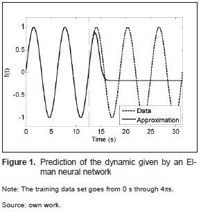
The target function in figure 1 is a perfect sine wave with period 2π and amplitude 1. Once the network has been trained, the output of the sys-tem has perfectly learned the data, which is in this case a set of samples from 0 to 4π seconds. The prediction looks well for a quarter of a period ahead, but as soon as the time at what the prediction is made overcomes that threshold the output of the system does not resemble the dynamic anymore. The network make a very soft interpolation of the sampling, which in this case correspond to 20 points per period, however when the input of the network is any time outside the training set then the prediction goes wrong. This experiment was repeated for the same target function, a pure sine wave, because it supposes to be an easy target. A large number of architectures were used, such as radial basis networks, cascade-forward backpropagation network, layered-recurrent network, feedforward backpropagation network, among many others. Also, a number of learning algorithms where tried, as well as different number of layers, and different neurons per layer. The conclusion is that a traditional neural network is not capable to generalize a periodic target function, thus why another type of network is tried in the next section.

3. Approximation By Fourier Neural Network

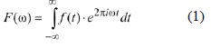
The literature review shows that one of the most common mathematical tools to deal with periodical functions is the Fourier expansion, which is an approximation used to rebuild curves based on sinusoidal signals. An associated tool is the Fourier transform, which is a function that takes functions in the time domain and converts them into the frequency domain, as is indicated in equation (1). The transformation has some advantages especially about the arithmetic, for instance derivatives can be seen as multiplications of the function by angular frequency (in the frequency domain). This property makes the transformation ideal to solve linear differential equations. The transformation is also used to observe some aspects of the signal that are hidden in the time domain or that are hard to see, such as harmonic content.

A result that comes from the Fourier transform is exclusively applied to periodic functions. This says that a periodic function can be approximated by a sum of sinusoidal signals with appropriated coefficients and frequencies, as shown in equation (2).

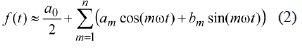
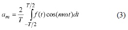
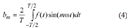
The target function is f(t), and a₀/2 is the mean value of the signal, ω is the angular frequency in rad/s. The frequency of the sinusoidal components in equation (2) are multiples of ω. The first value of mω, i.e., ω is called fundamental frequency, the second one, 2ω, is named second harmonic, and so on for other multiples. The coefficients a_m and b_m are computed as shown in equation (3) and equation (4)

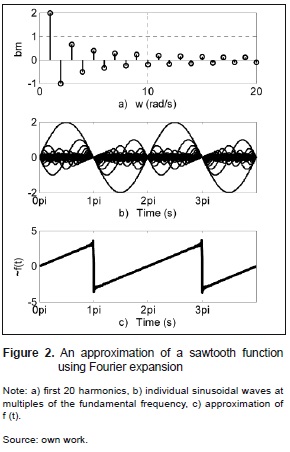
The result of the approximation of a sawtooth function using 128 harmonics is shown in figure 2. The symmetry of the function makes all coefficients a_m zero. The first part of the figure indicates the number of the harmonic in the x axis, and the value of the coefficient in the y axis. The intermediate figure shows every harmonic plotted in the time domain; the biggest signal is the fundamental signal with amplitude equal to two. The lower part of the figure is the sum of all the harmonics, and that is the approximation of the target function.

The work in [8] says that neural networks are good candidates to approximate dynamical systems. Three examples are presented in which the feedforward neural networks are used to approximate autonomous systems. The second work proves that a neural network with a unique neuron in the hidden layer can learn the Fourier transform of any function [9]; however nothing is said about the Fourier expansion. The third work says that a sinusoidal activation function improves the generalization of a neural network and this result is applied in problems called statistically neutral [10]. Those problems can be always reduced into two variables, and both variables have the same probability of occurrence. According to the work in [11], the coefficients of the Fourier expansion can be learned by a Hopfield neural network.

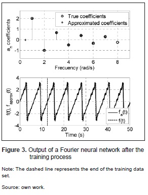
References [9], [10] and [11] are particularly important, because they show that the implementation of a feedforward neural network do learn a Fourier expansion. For the current application, that network has one input, the time, and one output, the prediction of the function value at the time indicated by the input. The network has only one hidden layer and the activation function is sinusoidal. This setup guarantees that the weights of the network, between input and hidden layer, are multiples of the fundamental frequency, whereas the weights between hidden layer and output are the coefficients of the Fourier expansion. The activation function of the output neuron is a linear function. Bias signal for every neuron is fixed on zero to reproduce the sine terms of the expansion, and π/2 for the terms associated with cosine. Bias of the output neuron is the average value of the function. The mathematical form of the neural network is shown in equation (5).

The comparison between the Fourier neural network in equation (5) and the Fourier expansion in equation (2) shows that b₀ is equivalent to a₀/2; also ω _n to mω; and b_n to 0 or π/2; finally, a_n in equation (5) is equivalent to the coefficients a_n y b_n in equation (2).

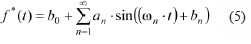
Once the architecture of the Fourier neural network has been defined, as is indicated in equation (5), the remaining work is to train the net based on the data set. The chosen training algorithm is the modified backpropagation Levenberg-Marquardt. One of the best results is shown in figure 3.

The Fourier neural network in figure 3 is trained using 100 data points per period, and the target function is a sawtooth function. The training data covers two periods. The validation of the training is made using the next eight periods. The lower part in figure 3 shows the target function and the approximation given by the network. The coefficients of the Fourier expansion as well as the approximations are plotted in the higher part in figure 3. The result in figure 3 looks promising but actually it is not. The prediction is very good for times smaller than or equal to the validation time window, but the prediction degenerates as the time increases. This problem is associated with the error allowed by the coefficients and multiples of the fundamental frequency.

The error on the parameters after the learning process has two sources: errors in magnitude, and errors in frequency. The analysis of these errors leads to say that errors on the frequency computation influence the approximation more than the errors on magnitude. A study of the deviation of the frequency is shown in figure 4. That example in figure 4a shows a target function compounds by two sinusoidal signals: one with unitary frequency and the other with frequency equal to 2 rad/s.

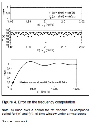
If the root mean square error RMSE for the two functions f₁(t) and f₂(t) is compared, is clear that the error is zero for ω₂ = 2, and one else where. No matter how close the value of ω₂ is, the error is there, except for ω₂ = 2. Then, if ω₂ is not the exact value then sooner or later the approximation will reach the maximum RMSE, and will come up with errors as bad as any other approximation. A derived result from figure 4.a is that the period of the combination f₁(t) and f₂(t) has a period that last about 10⁴ seconds, and its value is two only when ω₂ is exactly equal to 2. Even thought good approximations will remain good for more time than coarser approximations. Figure 4.c shows a window for the prediction, which is useful to define how long the approximation will be under certain RMSE, for example, in figure 4.c. that RMSE is 0,2 and the correspondent time is 493 s. Every approximation later than 493 s has RMSE bigger than 0,2.

4. Approximation of The fundamental frequency

The problem about approximating the fundamental frequency or its multiples using the Fourier Neural Network is that regardless of how close the estimation is the prediction gets worse and worse as the time goes. The next analysis has as a goal to answer why the learning algorithm, in this case backpropagation, causes that error. The answer is that the problem is precisely to minimize the RMSE, as shown in figure 5. To understand the problem let suppose that the data set has only two points t = 0 and t = 2π, and both are equal to one, because they come up from a square function with period 2π and amplitude equal to one. The analysis stars with the approximation given by only one harmonic, the fundamental frequency. The minimization of the RMSE is equivalent to find the sinusoidal that minimizes the distance between the data points and the harmonic.

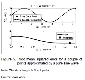
The first observation coming out from the result in figure 5 is that it is not possible to fix the error at zero, due to the difference in value between the approximation and the data at t = 0; and that difference happens regardless of the number of data points in the sampling. The second observation is about the frequency that minimizes the error: that frequency is different than the true frequency, regardless of the number of data points, and it happens even if the sampling contains the true period. That is because backpropagation minimizes the RMSE, then no matter how finer the sampling is the true frequency will not ever be reached, as shown by an asterisk in figure 5. For the next experiment the data set has a sampling rate of one data point per period across 64 periods, as it is shown in figure 6.

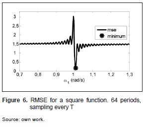
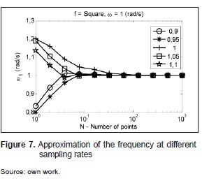
The good news about using more data is that the minimum gets closer to the true frequency value, so the minimization of the RMSE will get a better approximation if the data length is increased. Another characteristic is that the sampling does not need to match the true period, as shown in figure 7. The value 0,9 in figure 7 means than the sampling has been taken every 0,9 periods. The frequency that minimize the RMSE using just a couple of data points is within 10 % above and under the true value, in addition, as the quantity of data increases the maximum error shrinks, and makes the estimation closer to the true frequency. All the curves tend to 1 rad/s as the number of data points grows, it is the true frequency.

There are two problems that come from approximating the frequency if that is made by minimizing RMSE. The first one is that the error depends on the distribution of the samplings, in other words, different target functions require different amounts of data to get the same approximation; and the second problem is the learning algorithm itself, because it makes a search of the local minima from an initial guess and gets stack at a local minimum that is not necessarily the desired one, so the initial estimation to start with the minimization is quite critical. The second problem is detailed in figure 8 for a sawtooth target function. All cases were simulated using 15 points per period; the lower curve represents RMSE when the data set has 15 points, it is one period, and subsequent curves are simulation for an increasing data set at the same sampling rate, so the length of the next curve is two periods, 4, 8, and finally 16 for the highest curve.

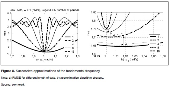
The number of local minima in figure 8 is incremented as the data increases, as is shown also in figure 6. Then, the strategy starts with few data points, where the number of local minima is low. Then, the data set is enlarged iteratively, and once a local minimum is reached for the first iteration, the data is incremented, for instance, to the double. In the next step the initial frequency for the enlarged data set is the same frequency that minimized RMSE in the first stage of the algorithm. This algorithm is repeated as far as it is necessary or data available.

5. Mathematical facts about The approximation

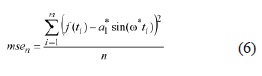
What is next is to prove mathematically that the minimization process already described certainly provides an approximation of the fundamental frequency, regardless of what the target function is. The root mean squared error between a function f(t) and a sinusoidal wave with amplitude a1* and frequency ω* in discrete time is given in equation (6):

Lemma 1

The minimization of the RMSE does not result in the fundamental frequency, regardless of the number of data points used to approximate the period.

The mean squared error in continuous time is defined in equation (7).

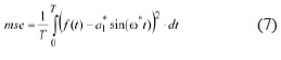
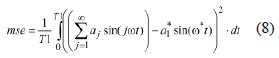
When n →∞, then mse_n → MSE, as Riemman sum says. In particular T in equation (7) can be T1 = (2π)/ω*. If the function f(t) is periodic, and in order to simplify the algebra, f(t) can be shifted back, so the first component of the Fourier expansion is completely sinusoidal. From now on, and looking for simplicity, the proof will be made for target function that can be written as a sum of sinusoidal waves exclusively. The Fourier expansion in equation (7) can be written as is shown in equation (8).

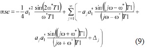
The computation of the integral is described in equation (9).

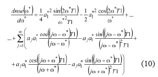
The variable ∆j represents all the independent terms of ω*. The derivative dmse(ω*)/dω* is computed in equation (10) to find the frequency ω* that minimize the root mean squared error.

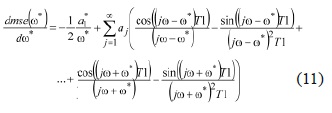
Since T1 = (2π)/ω*, then in equation (11):

The limit of ω* → ω. Using l'Hôpital's rule in equation (12) and equation (13) is: ... ...

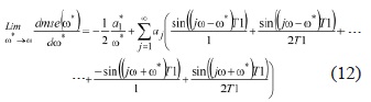
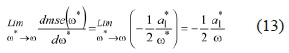
Since the limit of ω* → ω for dmse(ω*)/dω* is different than zero, then the minimum MSE shows up at ω* = ω, when T = T1. So, we can conclude that minimizing the MSE, the ω* will not be ω at T = T1.

Lemma 2:

In the limit when T → ∞ the frequency ω* → ω

The value of T1 from equation (11) will be re-place for Tz to simplify the analysis, so Tz = Z*T1 + T1/8, and Z is the set of natural numbers.

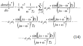
To simplify equation (14) in equation (15) the l'Hôpital's rule is applied to finde the limit when ω* → ω.

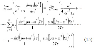
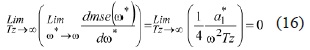
The conclusion is that ω* in equation (16) gets closer a closer to the true ω when Z → ∞.

Lemma 3:

The number of local minima of the RMSE around the fundamental frequency increases as the length of data set increases.

Let remember equation (11), but instead of T1 let use NT1 in equation (17) and equation (18), where N is a natural number.

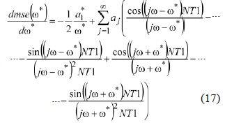
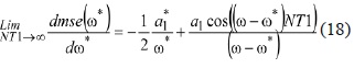
Since T1 = 2π/ω*, and the minimum for RMSE shows up at dmse(ω*)/dω* = 0, then in equation (19):

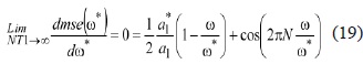
The result to remark so far happens when N → ∞, for this case the frequency of the cosine term grows linearly with N, so the number of local minima increases. The minimization of the MSE using backpropagation will get stack at the closest local minimum from the initial point of the search, and that initial frequency not necessarily is the one that makes the algorithm to halt at the minimum with a value closest to the true frequency. The limit of NT1 →∞ is ω* ≠ω, as it is shown in equation (19).

6. Results

The result of the three lemmas can be extended for an approximation of the second harmonic, in other words, when the minimization of the MSE estimates the double of the fundamental frequency. The intuitive idea is that a signal of period T is also periodic for an integer multiple of T, then if the data set has two periods, the approximation will provide two outputs, one close to T and another one close to 2T, and so on for any number of periods. The motivation for this intuitive idea is that instead of making approximations with one pure sinusoidal signal it is possible to use another signal, also periodic, with a shape like the function that is going to be approximate. The similarity between signals can be understood as the smallest distance, using any metric, between the harmonics of the true target and the approximant function.

If the number of terms for the approximant function is one, as it is shown in equation (20), the function is a sinusoidal wave, and its amplitude is one, in the same way that has been shown so far. If m is 2 then the approximation has 2 sinusoidal waves, and one has the double frequency of the other one, and so on.

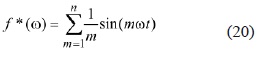
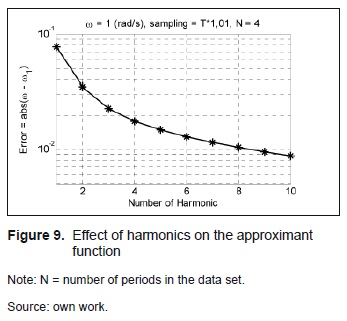
The difference between using only a sinusoidal wave and several harmonics looks subtle, but the result is remarkable. The number of data points required to make any approximation is reduced as it is shown in figure 9. For the experiment in figure 9 the sampling rate is 1,01T of a square signal, and the data set has only four data points. The x axis corresponds to the number of harmonics, n, and the result indicates that increasing the number of harmonics, leaving the number of data points fixed, improves the approximation. When the multiples of a sinusoidal wave are included in the approximant, the size of the expression in equation (20) increases and this has a computational cost; however the requirements for the length of the data sets are reduced. It seems that combining the two strategies is a good way to deal with the approximation problem. The procedure requires to increase the number of data points per period, and to increase the number of periods in the data set, and also to increase the number of harmonics in an iterative process in order to avoid undesirable local minima.

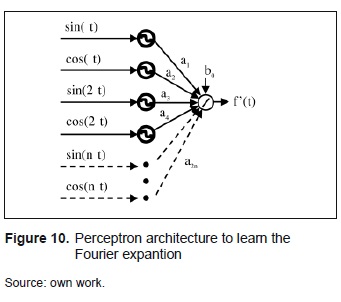
Once the frequency has been approximated, the approximation is used to train the Fourier neural network as it is shown in equation (5). The fundamental frequency and its multiples will be given by the approximation algorithm; in the same way as it is shown in figure 3. The network is the perceptron shown in figure 10. That architecture has an additional advantage: the phase angle that was required to learn in quation (5) is not required anymore, so the new goal is exclusively to learn the coefficients of the Fourier expansion using the weights of the network. By definition the coefficient of the Fourier expansion minimizes the mean square error, so running backpropagation, which minimizes MSE, is an ideal way to find the coefficient.

Experiments show that the modified backpropagation algorithm called Levenberg-Marquardt gets stable after just one epoch; however there is an error on the value of the coefficients, they are just approximations. Even though, increasing the number of data points per period, it is refining the sampling improves the approximation. Results of the estimation of a triangular function are shown in figure 11. The approximation of the frequency used for running this experiments is 1,0001, and the true value is 1 (rad/s).

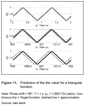
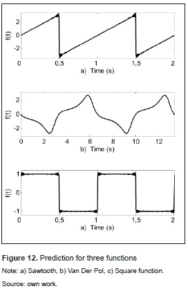
The prediction in figure 11 is very close to the true target for low values of time; and even after 500 seconds, which are 500 periods of the function, the approximation is relatively good; even thought the error is visible at times like 1000 s. The approximations for other three types of function are shown in figure 12. The results are better for smooth functions like the oscillator, because of the effect well known as Gibbs phenomenon; this condition predicts problems around the discontinuities.

7. Conclusions

The reconstruction of periodic signals can be performed by approximating the period of the signal, which can be seen also as a approximating the fundamental frequency. This frequency is estimated using a single neuron with a sine transfer function and backpropagation as training algorithm. The approximation leads to an inevitable error that can be minimized only increasing the amount of data in an iterative fashion. This paper presents an algorithm that smartly uses data samples, evenly spaced, to approximate the period of a signal trough successive iterations. The first iteration requires a rough approximation of the period and data points to cover at least the guessed period, and then the minimization of the mean squared error provides a first estimation for the period. The estimation at the end of each iteration is used as the initial guess for the next iteration, at the same time, the data length is progressively increased every iteration, which guarantee that the next iteration will provide a better approximation than the previous one. This paper includes the mathematical proof about the quality of the estimation, and in addition proposes a first modification of the algorithm to reduce the amount of data required to make the estimation, which is by means of approximating not only the fundamental frequency, but also the harmonics. Once the period is estimated, then a perceptron network can be used to approximate the Fourier coefficients, which serves to reconstruct the entire dynamic of a periodic system. Future works could study ways to reduce the quantity of data require for the algorithm, and also ways to validate the results of the algorithm for quasi periodic signals.

References

[1] R. G. McKilliam, B. G. Quinn, I. V. L. Clarkson, and B. Moran, "Frequency estimation by phase unwrapping", IEEE Trans. on Signal Processing, vol. 58, no. 6, pp. 2953-2963, Jun. 2010.

[2] S. Provencher, "Estimation of complex single-tone parameters in the DFT domain", IEEE Trans. on Signal Processing, vol. 58, no. 7, pp. 3879-3883, Jul. 2010.

[3] H. C. So, and F. K. W. Chan, W. Sun, "Subspace approach for fast and accurate single-tone frequency estimation", IEEE Trans. on Signal Processing, vol. 59, no. 2, pp. 827-831, Feb. 2011.

[4] R. Chudamani, K. Vasudevan, and C. S. Ramalingam, "Real-time estimation of power system frequency using nonlinear least squares", IEEE Trans. on Power Delivery, vol. 24, no. 3, pp. 1021-1028, Jul. 2009.

[5] Y. Pantazis, O. Rosec, and Y. Stylianou, "Iterative estimation of sinusoidal signal parameters", IEEE Signal Processing Letters, vol. 17, no. 5, pp. 461-464, May. 2010.

[6] C. Candan, "A method for fine resolution frequency estimation from three DFT samples", IEEE Trans. on Signal Processing Letters, vol. 18, no. 6, pp. 351-354, Jun. 2011.

[7] C. Yang, and G. Wei, "A noniterative frequency estimator with rational combination of three spectrum lines", IEEE Trans. on Signal Processing, vol. 59, no. 10, pp. 5065-5070, Oct. 2011.

[8] J. M. Rodríguez, and M. H. Garzón. "Neural Networks can learn to Approximate Autonomous Flows", Fluids and Waves: Recent Trends in Applied Analysis, University of Memphis, TN, vol. 440, 2007, pp. 197-205.

[9] A. Menon, K. Mehrotra, C. K. Mohan, and S. Ranka, "Characterization of a Class of Sigmoid Functions with Applications to Neural Networks", Elsevier Science Neural Networks, vol. 9, no. 5, pp. 819-835, Jul. 1996.

[10] A.A. Ghorbani, and K. Owrangh, "Stacked generalization in neural networks: generalization on statistically neutral problems", in Proc. of the International joint conference on Neural Networks IJCNN 2001, Washington USA, 2001, vol. 3, pp. 1715-1720.

[11] M. Karam, M. S. Fadali, and K. White, "A Fourier/Hopfield neural network for identification of nonlinear periodic systems", in Proc. of the 35th Southeastern Symposium on System Theory, Morgantown, WV, USA, 2003, pp. 53-57.