
DOI:
https://doi.org/10.14483/22487638.17131Publicado:
01-10-2021Número:
Vol. 25 Núm. 70 (2021): Octubre - DiciembreSección:
InvestigaciónMetodología para la síntesis de autómatas en la planificación de movimientos en sistemas autónomos con múltiples agentes
Methodology for the Synthesis of Automata in the Planning of Movements for Autonomous Systems with Multiple Agents
Palabras clave:
Büchi automata, formal languages, linear temporal logic (LTL), motion planning, Petri networks (en).Palabras clave:
autómatas de Büchi, lenguajes formales, lógica temporal lineal (LTL), , planificación de movimientos, redes de Petri, sistemas cooperativos de múltiples agentes (es).Descargas
Referencias
Aksaray, D., Jones, A., Kong, Z., Schwager, M., & Belta, C. (2016). Q-learning for robust satisfaction of signal temporal logic specifications. 2016 IEEE 55th Conference on Decision and Control (CDC), 6565-6570. https://doi.org/10.1109/ACC.2012.6315110 DOI: https://doi.org/10.1109/CDC.2016.7799279
Aragues, R., Shi, G., Dimarogonas, D. V, Sagues, C., & Johansson, K. H. (2012). Distributed algebraic connectivity estimation for adaptive event-triggered consensus. American Control Conference (ACC), 2012, 32-37. DOI: https://doi.org/10.1109/ACC.2012.6315110
Brown, F. M. (2012). Boolean reasoning: the logic of Boolean equations. Springer Science & Business Media.
Chen, Y., Ding, X. C., Stefanescu, A., & Belta, C. (2012). Formal approach to the deployment of distributed robotic teams. IEEE Transactions on Robotics, 28(1), 158-171. https://doi.org/10.1109/TRO.2011.2163434 DOI: https://doi.org/10.1109/TRO.2011.2163434
Choset, H. M. (2005). Principles of robot motion: theory, algorithms, and implementation. MIT press.
Clarke, E. M., Grumberg, O., & Peled, D. (1999). Model checking. MIT press.
Costelha, H., & Lima, P. (2012). Robot task plan representation by Petri nets: modelling, identification, analysis and execution. Autonomous Robots, 33(4), 337-360. https://doi.org/10.1007/s10514-012-9288-x DOI: https://doi.org/10.1007/s10514-012-9288-x
Ding, X. C., Kloetzer, M., Chen, Y., & Belta, C. (2011). Automatic deployment of robotic teams. IEEE Robotics & Automation Magazine, 18(3), 75-86. https://doi.org/10.1109/MRA.2011.942117 DOI: https://doi.org/10.1109/MRA.2011.942117
Ding, X. C., Smith, S. L., Belta, C., & Rus, D. (2014). Optimal Control of Markov Decision Processes With Linear Temporal Logic Constraints. IEEE Transactions on Automatic Control, 59(5), 1244-1257. https://doi.org/10.1109/TAC.2014.2298143 DOI: https://doi.org/10.1109/TAC.2014.2298143
Emerson, E. A. (1990). Temporal and modal logic. In J. van Leeuwen (Ed.) Handbook of Theoretical Computer Science, Volume B: Formal Models and Sematics (B) (pp. 995, 997-1072). Elsevier. https://doi.org/10.1016/B978-0-444-88074-1.50021-4 DOI: https://doi.org/10.1016/B978-0-444-88074-1.50021-4
Franceschelli, M., Giua, A., & Pisano, A. (2014, June 4-6). Finite-time consensus on the median value by discontinuous control [Conference presentation]. American Control Conference (ACC), 2014, Portland, OR, USA. https://doi.org/10.1109/ACC.2014.6859201 DOI: https://doi.org/10.1109/ACC.2014.6859201
Franceschelli, M., Rosa, D., Seatzu, C., & Bullo, F. (2013). Gossip algorithms for heterogeneous multi-vehicle routing problems. Nonlinear Analysis: Hybrid Systems, 10, 156-174. https://doi.org/10.1016/j.nahs.2013.03.001 DOI: https://doi.org/10.1016/j.nahs.2013.03.001
Garrido, S., Moreno, L., Gómez, J. V, & Lima, P. U. (2013). General path planning methodology for leader-follower robot formations. International Journal of Advanced Robotic Systems, 10(1), 64. https://doi.org/10.5772/53999 DOI: https://doi.org/10.5772/53999
Gastin, P., & Oddoux, D. (2001). Fast LTL to Büchi automata translation. In G. Berry, H. Comon, & A. Finkel (Eds.) Computer Aided Verification. CAV 2001. Lecture Notes in Computer Science (vol. 2102, pp. 53-65). Springer. https://doi.org/10.1007/3-540-44585-4_6 DOI: https://doi.org/10.1007/3-540-44585-4_6
Guo, M., & Dimarogonas, D. V. (2015a). Multi-agent plan reconfiguration under local LTL specifications. The International Journal of Robotics Research, 34(2), 218-235. https://doi.org/10.1177/0278364914546174 DOI: https://doi.org/10.1177/0278364914546174
Guo, M., & Dimarogonas, D. V. (2015b, August 24-28). Bottom-up motion and task coordination for loosely-coupled multi-agent systems with dependent local tasks [Conference presentation]. 2015 IEEE International Conference on Automation Science and Engineering (CASE), Gothenburg, Sweden. https://doi.org/10.1109/CoASE.2015.7294103 DOI: https://doi.org/10.1109/CoASE.2015.7294103
Holzmann, G. (2003). Spin model checker, the: primer and reference manual. Addison-Wesley Professional.
Martínez-Valencia, J. L., Holguín-Londoño, M., & Escobar-Mejía, A. (2017, October 18-20). A methodology to evaluate combinatorial explosion using LTL in autonomous ground navigation applications [Conference presentation]. 2017 IEEE 3rd Colombian Conference on Automatic Control (CCAC), Cartagena, Colombia. https://doi.org/10.1109/CCAC.2017.8276430 DOI: https://doi.org/10.1109/CCAC.2017.8276430
Karaman, S., & Frazzoli, E. (2011). Linear temporal logic vehicle routing with applications to multi-UAV mission planning. International Journal of Robust and Nonlinear Control, 21(12), 1372-1395. https://doi.org/10.1002/rnc.1715 DOI: https://doi.org/10.1002/rnc.1715
Karaman, S., & Frazzoli, E. (2009, December 15-18). Sampling-based motion planning with deterministic $μ$-calculus specifications [Conference presentation]. 48h IEEE Conference on Decision and Control (CDC) held jointly with 2009 28th Chinese Control Conference, Shanghai, China. https://doi.org/10.1109/CDC.2009.5400278 DOI: https://doi.org/10.1109/CDC.2009.5400278
Kloetzer, M., & Mahulea, C. (2014). A Petri net based approach for multi-robot path planning. Discrete Event Dynamic Systems, 24(4), 417-445. https://doi.org/10.1007/s10626-013-0162-6 DOI: https://doi.org/10.1007/s10626-013-0162-6
Kloetzer, M., & Mahulea, C. (2015). Ltl-based planning in environments with probabilistic observations. IEEE Transactions on Automation Science and Engineering, 12(4), 1407-1420. https://doi.org/10.1109/TASE.2015.2454299 DOI: https://doi.org/10.1109/TASE.2015.2454299
Kloetzer, M., & Mahulea, C. (2016, May 30-June 1). Multi-robot path planning for syntactically co-safe LTL specifications [Conference presentation]. 13th International Workshop On Discrete Event Systems (WODES), Xi'an, China. https://doi.org/10.1109/WODES.2016.7497887 DOI: https://doi.org/10.1109/WODES.2016.7497887
Kupferman, O., & Vardi, M. Y. (2001). Model checking of safety properties. Formal Methods in System Design, 19(3), 291-314. https://doi.org/10.1023/A:1011254632723 DOI: https://doi.org/10.1023/A:1011254632723
LaValle, S. M. (2006). Planning algorithms. Cambridge university press. DOI: https://doi.org/10.1017/CBO9780511546877
Ma, X., Jiao, Z., Wang, Z., & Panagou, D. (2016, June 7-10). Decentralized prioritized motion planning for multiple autonomous UAVs in 3D polygonal obstacle environments [Conference presentation]. 2016 International Conference on Unmanned Aircraft Systems (ICUAS), Arlington, VA, USA. https://doi.org/10.1109/ICUAS.2016.7502596 DOI: https://doi.org/10.1109/ICUAS.2016.7502596
Mahulea, C., & Kloetzer, M. (2014, December 15-17). Planning mobile robots with Boolean-based specifications [Conference presentation]. 2014 IEEE 53rd Annual Conference on Decision and Control (CDC), Los Angeles, CA, USA. https://doi.org/10.1109/CDC.2014.7040192 DOI: https://doi.org/10.1109/CDC.2014.7040192
Martínez, J. L., Holguín, G. A., & Holguín, M. (2018, November 1-3). A Methodology for Movement Planning in Autonomous Systems with Multiple Agents [Conference presentation]. 2018 IEEE 2nd Colombian Conference on Robotics and Automation (CCRA), Barranquilla, Colombia. https://doi.org/10.1109/CCRA.2018.8588140 DOI: https://doi.org/10.1109/CCRA.2018.8588140
Piterman, N., Pnueli, A., & Sa’ar, Y. (2006, January 8-10). Synthesis of reactive (1) designs [Conference presentation]. International Workshop on Verification, Model Checking, and Abstract Interpretation, Charleston, SC, USA. https://doi.org/10.1007/11609773_24 DOI: https://doi.org/10.1007/11609773_24
Pnueli, A., & Rosner, R. (1989, January 11-13). On the synthesis of a reactive module [Conference presentation]. 16th ACM SIGPLAN-SIGACT Symposium on Principles of Programming Languages, Austin, TX, USA. https://doi.org/10.1145/75277.75293 DOI: https://doi.org/10.1145/75277.75293
Saha, I., Ramaithitima, R., Kumar, V., Pappas, G. J., & Seshia, S. A. (2014, September 14-18). Automated composition of motion primitives for multi-robot systems from safe LTL specifications [Conference presentation]. 2014 IEEE/RSJ International Conference on Intelligent Robots and Systems, Chicago, IL, USA. https://doi.org/10.1109/IROS.2014.6942758 DOI: https://doi.org/10.1109/IROS.2014.6942758
Schillinger, P., Bürger, M., & Dimarogonas, D. (2016, November 6-9). Decomposition of Finite LTL Specifications for Efficient Multi-Agent Planning [Conference presentation]. 13th International Symposium on Distributed Autonomous Robotic Systems, London, UK.
Smaus, J.-G. (2007, May 23-26). On Boolean functions encodable as a single linear pseudo-Boolean constraint [Conference presentation]. International Conference on Integration of Artificial Intelligence (AI) and Operations Research (OR) Techniques in Constraint Programming, Brussels, Belgium. https://doi.org/10.1007/978-3-540-72397-4_21 DOI: https://doi.org/10.1007/978-3-540-72397-4_21
Tumova, J., & Dimarogonas, D. V. (2015, December 15-18). Decomposition of multi-agent planning under distributed motion and task LTL specifications [Conference presentation]. IEEE 54th Annual Conference on Decision and Control (CDC), Osaka, Japan. https://doi.org/10.1109/CDC.2015.7403396 DOI: https://doi.org/10.1109/CDC.2015.7403396
Ulusoy, A., Smith, S. L., Ding, X. C., & Belta, C. (2012, May 12-14). Robust multi-robot optimal path planning with temporal logic constraints [Conference presentation]. IEEE International Conference on Robotics and Automation (ICRA), Saint Paul, MN, USA. https://doi.org/10.1109/ICRA.2012.6224792 DOI: https://doi.org/10.1109/ICRA.2012.6224792
van den Berg, J. P., & Overmars, M. H. (2005, August 2-6). Prioritized motion planning for multiple robots [Conference presentation]. 2005 IEEE/RSJ International Conference on Intelligent Robots and Systems, Edmonton, AB, Canada. https://doi.org/10.1109/IROS.2005.1545306 DOI: https://doi.org/10.1109/IROS.2005.1545306
Wolper, P., Vardi, M. Y., & Sistla, A. P. (1983, November 7-9). Reasoning about infinite computation paths [Conference presentation]. 24th Annual Symposium on Foundations of Computer Science, Tucson, AZ, USA. https://doi.org/10.1109/SFCS.1983.51 DOI: https://doi.org/10.1109/SFCS.1983.51
Wongpiromsarn, T., Topcu, U., & Murray, R. M. (2009, December 15-18). Receding horizon temporal logic planning for dynamical systems [Conference presentation]. 48th IEEE Conference on Decision and Control, 2009 Held Jointly with the 2009 28th Chinese Control Conference, Shanghai, China. https://doi.org/10.1109/CDC.2009.5399536 DOI: https://doi.org/10.1109/CDC.2009.5399536
Yen, J. Y. (1971). Finding the k shortest loopless paths in a network. Management Science, 17(11), 712-716. https://doi.org/10.1287/mnsc.17.11.712 DOI: https://doi.org/10.1287/mnsc.17.11.712
Cómo citar
APA
ACM
ACS
ABNT
Chicago
Harvard
IEEE
MLA
Turabian
Vancouver
Descargar cita
Recibido: 21 de octubre de 2020; Aceptado: 12 de agosto de 2021
ABSTRACT
Objective:
To present a methodology for motion planning in autonomous systems with multiple agents.
Methodology:
The physical behavior of a team of autonomous navigation systems is parameterized and defined. Then, a control policies algorithm is described and implemented, which interprets these descriptions, which are converted into LTL formulas, and a model is generated which allows making automatic abstractions. From generic solution configurations, the case of multiple robots with a single task in an environment with fixed obstacles is derived. The methodology is validated in different scenarios, and the results are analyzed.
Results:
The proposed methodology for motion planning in autonomous systems with multiple agents combines two state-of-the-art techniques, thus allowing to mitigate the combinatorial explosion of states in traditional approaches.
Conclusions:
The proposed methodology solves the automaton synthesis problem for high-level control with task changes during the execution. Under certain criteria, the problem of combinatorial explosion of states associated with these systems is mitigated. The solution is optimal with regard to the number of transactions performed by the team members.
Funding:
Universidad Tecnológica de Pereira
Keywords:
Büchi automata, formal languages, linear temporal logic (LTL), motion planning, Petri networks, cooperative systems with multiple agents.RESUMEN
Objetivo:
Presentar una metodología para la planificación de movimientos de sistemas autónomos con múltiples agentes.
Metodología:
Se define y parametriza el comportamiento físico de un equipo de sistemas de navegación autónoma. Luego se describe e implementa un algoritmo de síntesis de políticas de control que interpreta estas descripciones convertidas a fórmulas LTL y se genera un modelo que permite hacer abstracciones automáticas. A partir de configuraciones genéricas de solución, se deriva en el caso de múltiples robots con una única tarea en un entorno con obstáculos fijos. La metodología se valida en diferentes escenarios y se analizan los resultados.
Resultados:
La metodología propuesta para planificación de movimientos en sistemas con múltiples agentes combina dos técnicas del estado del arte, permitiendo mitigar la explosión combinacional de estados presente en los enfoques tradicionales.
Conclusiones:
La metodología que se presenta resuelve el problema de síntesis de autómatas para el control de alto nivel, con cambio de tareas durante la ejecución. Bajo ciertos criterios, se mitiga el problema de explosión combinacional de estados asociado a estos sistemas. La solución es óptima respecto al número de transiciones seguidas por los miembros del equipo.
Financiamiento:
Universidad Tecnológica de Pereira
Palabras clave:
autómatas de Büchi, lenguajes formales, lógica temporal lineal (LTL), planificación de movimientos, redes de Petri, sistemas cooperativos de múltiples agentes.INTRODUCTION
With the great advances in the technology that supports autonomous systems, the variety of tasks for which they may be required has also expanded. This has aroused the particular interest of the scientific community in solving movement planning problems in autonomous systems, focusing on calculating the necessary trajectories for a system to fulfill a task (Choset, 2005; LaValle, 2006).
This problem has been studied, not only for the case of an autonomous system, but also for the case of multiple agents (Ding et al., 2014; Franceschelli et al., 2013). Most of the existing works that carry out this type of tasks lack the expressiveness to capture the requirements (Ma et al., 2016; van den Berg & Overmars, 2005), they are based on simplifying the abstractions, which results in a conservative behavior (Aksaray et al., 2016), or they do not consider the time restrictions in the execution of the task (Saha et al., 2014). In addition to these limitations, many of the planning methods are computationally intractable (and therefore do not scale well or work in real-time) and provide guarantees only in a simplified abstraction of system behavior (Aksaray et al., 2016).
One of the main challenges in this area is the development of a computationally efficient framework that meets the physical constraints of the robot and the complexity of the environment while allowing a broad spectrum of task specifications (Ding et al., 2011). Some authors suggest that, by using linear temporal logic (LTL), such as the task specification language, the flexibility to incorporate explicit time constraints is preserved, as well as a variety of behaviors (Clarke et al., 1999), i.e., LTL can be used as a rich specification language in autonomous systems such as mobile robotics (Karaman & Frazzoli, 2009; Wongpiromsarn et al., 2009). LTL is often found as a formalism to express high-level tasks for autonomous systems (Ding et al., 2014; Guo & Dimarogonas, 2015a; Kloetzer & Mahulea, 2015), and such tasks can refer to a single robot (Ding et al., 2014), specify individual requirements for mobile robots (Guo & Dimarogonas, 2015a), or impose a global specification for robotic equipment (Kloetzer & Mahulea, 2015). In Kloetzer and Mahulea (2016) an iterative algorithm is proposed which plans the movements of a team of robots that unfolds in a workspace modeled as a Petri net. The main part of the algorithm is represented by specific mathematical programming formulations that produce trajectories for the robots, without considering the collisions between them. Petri nets have been used previously in different robotic problems, for example, in Costelha and Lima (2012) to model the real execution of the movement plan, in Kloetzer and Mahulea (2014) to solve accessibility problems under probabilistic information, or in Mahulea and Kloetzer (2014) to satisfy the tasks given as Boolean formulas. In a multi-robot configuration, Guo and Dimarogonas (2015b) propose a bottom-up approach to plan actions, given an LTL specification for each robot. In Karaman and Frazzoli (2011) the routing problem of a vehicle with LTL restrictions is expanded, and a solution based on Mixed Integer Linear Programming (MILP) is planned. In Ulusoy et al. (2012) and Chen et al. (2012), a single mission is assumed for a robotic team, and “trace-closed” languages are used to distribute the mission, but possible collisions are not considered between robots.
Computational complexity is still a major challenge in planning multi-robot systems. To reduce complexity, in Tumova and Dimarogonas (2015), summaries of independent movements of individual agents are made; and, in Schillinger et al. (2016), a way to identify independent parts of a given mission is proposed as a finite LTL formula. Some works have proposed algorithmic solutions for movement planning problems in various scenarios, such as synthesis of high-level tasks (Guo & Dimarogonas, 2015a; Kloetzer & Mahulea, 2015), consensus problems (Aragues et al., 2012; Franceschelli et al., 2014), and leading follower (Garrido et al., 2013).
Therefore, from the above, the objective of this work is to present a methodology for planning the movements of autonomous systems with multiple agents. The methodology is validated in different scenarios and the results are analyzed.
PRELIMINARIES
Büchi automata
A Büchi automaton corresponding to an LTL formula on set Π has the structure B=(S,S0,ΣB,→B,F), where:
-
S is a finite set of states
-
S0⊆ S is the set of initial states
-
ΣB=2Π is the input character set
-
→B⊆ S×ΣB×S is the transition relation
-
F ⊆ S is the set of final states
For si, sj ∈ S, ρ(si,sj) is the set of all entries in B that allow the transition from si to sj. The transitions in B can be non-deterministic, which means that, from a given state, there can be multiple outgoing transitions enabled by the same input, that is, it can be stated that (s,τ,s′) ∈→B and (s,τ,s′′) ∈→B with s′≠s′. Therefore, an input sequence can produce more than one sequence of output states. A non-deterministic finite automaton can be made deterministic, but, in this case, a non-deterministic automaton is preferable given the lower number of states. An infinite input word, that is, a sequence of elements of Σ_B, is accepted by B if the word produces at least one sequence of states of B, which, when traversed, allow visiting the future state of the set F.
Petri nets
There are multiple known configurations of Petri nets (RdP), and their application to modeling movements in robotic systems is of interest. This type of RdP system for robot movement (RMPN) is a quadruple Q = (N, m0, ∏, h), where:
-
N = (P, T, Post, Pre) is the structure of the RdP with P being the set of places.
-
T is the set of transitions modeling the possibilities of movement of the robots between the places; Post ∈ {0,1} ^ (| P | × | T |) is the post-incidence matrix defining the arcs of the transitions to the places, and Pre ∈ {0,1} ^ (| P | × | T |) is the pre-incidence matrix defining the arcs of the places to the transitions. ∀t∈T, | • t | = | t • | = 1, where • t and t • are the set of inputs and outputs of the t places (• t = {p∈P | Pre [p, t]> 0} and t • = {p∈P | Post [p, t]> 0}).
-
Π∪{∅} is the output alphabet, where ∅ denotes an empty observation.
-
h:P→2Π is the observation map, where 2Π is the set of all subsets of Π, including the empty set ∅, and h(pi) produces the output of the place
-
pi ∈ P. If pi has at least one mark, then the propositions of h(pi) are active.
Linear temporal logic (LTL)
The syntax to construct the π formulas can be defined recursively according to the following grammar (Piterman et al., 2006): φ∷ = π | ¬φ | φ∨φ | ∘φ | φuφ. Starting from the previous grammar, it is known that the Boolean constants True and False are defined as True = (φ∨¬φ) and False = ¬True. From the negation (¬) and the disjunction (∨), we can define the conjunction (∧), the implication (→), and the equivalence (↔). Furthermore, by counting in the grammar with the temporary operators "next" (∘) and "until" (U), additional temporary operators such as "Eventually" (⋄φ = True Uφ) and "always" (□ φ = ¬⋄¬φ) can be used. The semantics of an LTL formula φ are defined over an infinite sequence σ of assignments of truth to the atomic sentences π∈AP. Table 1 recursively defines σ, I⊧φ, where σ (i) is the set of atomic sentences that are true at position i. The formula ∘φ expresses that φ is true at the next position in the sequence (the next time state), and the formula φ_1 Uφ_2 expresses that φ_1 is true until φ_2 begins to be true. The sequence σ satisfies the formula φ if (σ, 0⊧φ). The sequence σ satisfies the formula □ φ if φ is true in all positions of the sequence. Furthermore, it satisfies the formula ⋄φ if φ is true in some position of the sequence. The sequence σ satisfies the formula □ ⋄φ if, at any position, φ becomes true, that is, φ frequently begins to be true infinitely. For a formal definition of LTL, see the work by Emerson (1990).
Source: Authors
Table 1: Recursive definition of semantics for LTL formulas
Relation
Definition
(𝜎,𝑖⊧𝜋)
IF (𝜋∈𝜎(𝑖))
(𝜎,𝑖⊧¬𝜑)
IF (𝜎,𝑖¬⊧𝜑)
(𝜎,𝑖⊧𝜑1∨𝜑2)
IF (𝜎,𝑖⊧𝜑1) 𝑜𝑟 (𝜎,𝑖⊧𝜑2)
(𝜎,𝑖⊧∘𝜑)
IF (𝜎,𝑖+1⊧𝜑)
𝜎,𝑖⊧𝜑1𝑈𝜑2
IF, in the future, there is a (𝑘≥𝑖) so that (𝜎,𝑘⊧𝜑2), and for every (𝑖≤𝑗≤𝑘) t (𝜎,𝑗⊧𝜑1)
Some of the properties that can be expressed using LTL are:
-
Reaching a target while avoiding obstacles (π1 ∨ π2 ∨…∨πn)Uπ, capturing the property that eventually π is going to be true and, until that happens, obstacles labeled πi;i = 1,2,…,must be avoided n.
-
Sequencing: ⋄(π1 ∧⋄(π2 ∧⋄ π3)) captures the requirement that the robot first visit the region π1, then the region π2 and then the region π3, respecting that order.
-
Coverage: ⋄π1 ∧⋄ π2 ∧…∧⋄ πm specifies that the robot will eventually reach π1, eventually reach π2, …, and eventually reach πm. The robot will at some point visit all regions of interest in any order.
Another particular class of LTL formula is known as syntactically co-safe formulas (Kupferman & Vardi, 2001). Any solution that satisfies a co-safe LTL formula consists of a finite string known as a good prefix, followed by an infinite continuation of statements, thus ensuring that this continuation does not affect the truth value of the formula. It was shown by Kupferman and Vardi (2001) that any LTL formula that contains only temporary operators ⋄ and U when written in positive normal form, that is, when the negation ¬ appears only before atomic sentences, is syntactically safe.
For this case of LTL formulas, the Büchi automaton, B, accepts an input word if it starts with a good finite prefix that takes B to the set of final states (the continuation of the prefix is irrelevant). Therefore, the satisfaction of the co-safe LTL formulas is decided based on the finite executions of the RMPN model defined in the next section.
METHODOLOGY
This section begins by defining and parameterizing the physical behavior of an autonomous navigation system equipment. Then, the control policy synthesis algorithm is described and implemented, which interprets the descriptions previously converted to LTL formulas, and, based on these specifications, it generates a model that allows automatic abstractions, thus guaranteeing that said model allows meeting the specifications given for the environment. Some of the solution configuration possibilities for the proposed problem are considered, and a different case is evaluated for each one, thus defining the case of a single robot located in an environment with fixed or mobile obstacles, and the case of multiple robots with a single task located in an environment with fixed obstacles modeled through a Petri net. Finally, a series of simulations is proposed which allows validating the proposed methodology in the different scenarios and comparing the results obtained.
Definition and parameterization of a team of autonomous land navigation systems
It is assumed that the type of mobile robots used operates in a polygonal workspace P. The movement of a robot is expressed by p ̇ (t) = u (t), p (t) ∈P⊆R, u (t) ∈U⊆R ^ 2, where p (t) is the robot's position at time t, and u (t) is the control input. It is assumed that the workspace P is partitioned into a finite number of cells P_1,…, P_n, where P = ∪_ (i = 1) ^ n P_i and P_i∩P_j = Φ if i ≠ j. Furthermore, each of the cells is considered as a convex polygon. When partitioning the workspace, a series of Boolean statements r_1, r_2,…, r_n is generated, which is true if the robot is in position P_i. Then, the RMPN that models the work environment is automatically generated. A workspace like the one shown in Figure 1a is proposed, partitioned into five cells duly labeled as a_1,…, a_5, with two robots initially located at a_1 and a_5, and five regions of interest π_1, π_2, π_3 , π_4, π_5, so that region π_1 corresponds to cell a_1 and place p_1, region π_2 corresponds to a_2 and place p_2, and so on.
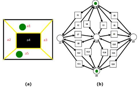
Figure 1: a) Workspace; b) modeling of a workspace through Petri nets
For the environment described above, an RMPN model is obtained which can be seen in Figure 1b, where P= p1,…,p5 and T=t1,…,t16. . Since the set of input transitions of p1 is •p1=t2,t4,t6, then Post[p1,t2]=Post[p1,t4]=Post[p1,t6]=1, while Post[p1,tj]=0 for all tj∈T\•p1. Furthermore, since the set of output transitions of p1 is p1• = t1,t3,t5, then Pre[p1,t1]=Post[p1,t5]=Post[p1,t7]=1, while Pre[p1,tj]=0 for all tj∈T\p1•..
Case 1 - a robot and multiple obstacles
A single robot is located in the workspace R shown in Figure 2, which is partitioned into 16 regions related to the location propositions of the robot R=r1,r2,…,r16, initially located in region 2, and with a specification given in natural language such as “Go from region 2 to region 15 and then back to region 2. If an obstacle is encountered on the road, turn on a light and stay in the same place until the obstacle disappears. If the obstacle disappears, turn off the light and get back on your way”.
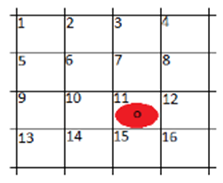
Figure 2: Workspace R
As the obstacles are part of the environment, the set of surveyed propositions contains only one proposition X = S ^ obs, which becomes true if the robot detects an obstacle. The assumptions about the obstacles are captured by φ_e = φ_i ^ e∧φ_t ^ e∧φ_g ^ e. Initially, the robot does not detect any obstacles; therefore, φ_i ^ e = (¬S ^ obs). It is assumed that the robot can only detect obstacles in regions other than region 2 and region 15, so the restriction is coded in such a way that, in regions 2 and 15, the value of S ^ obs cannot change. This requirement is captured by the formula: φ_t ^ e = □ ((¬r_1∧¬r_3∧… ∧¬r_13∧¬r_14∧¬r_16) → (∘S ^ obs↔S ^ obs)). Since no more hypotheses are assumed about the surrounding propositions, we have φ_g ^ e = (True).
Now, to model the robot and the desired specifications that are captured by φ_s = φ_i ^ s∧φ_t ^ s∧φ_g ^ s, 17 robot propositions are defined, which are expressed in Y = r_1, r_2, r_16, a ^ (light_On) . As an initial location condition, the robot can start in region 2, or in region 15 with the light off, since, in these regions, there should be no obstacles. We then have the equation φ_i ^ s = {(r_2 ∧_i∈ {1, 3, 16} ¬r_i∧¬a ^ light On) ∨ (r_15 ∧_i∈ {1,…, 13,14,16} ¬ r_i∧¬a ^ (light_On)).
The formula φ_t ^ s is defined in Equation (3), and it models the possible changes in the state of the robot. The first block of sub-formulas that compose it represents the possible transitions between the regions. For example, from region 1, the robot can move to region 2, or to region 5, or it can remain in region 1. The following sub-formula represents the mutual exclusion constraint between regions that specifies that, at any one time, only one region of R can be true. The last block of sub-formulas represents the desired specifications for the system and establishes that, if the robot encounters an obstacle, it must remain motionless with the light on until it is removed, considering in turn that, if the robot does not encounter an obstacle, the light must be off. Finally, φ_g ^ s captures the requirement that the robot keep moving between regions 2 and 16, unless it encounters an obstacle. The synthesis of the problem consists of the construction of an automaton whose behaviors satisfy the formula φ. It is proven that the size of this automaton is equal to the double exponential of the size of the formula (Pnueli & Rosner, 1989). However, if the problem is restricted to the special class of LTL formulas GR (1), the algorithm introduced by Piterman et al. (2006) can be used, which is of polynomial time O (n ^ 3), where n is the size of the state space. In this case, each of the states corresponds to an assignment of admissible truth for the set of propositions of the environment and the robot.
The synthesis process is seen as a game between the robot and the environment, with the latter as the adversary. Starting from some initial state, the robot and the environment make decisions that determine the next state of the entire system. The condition to win the game is given by a class of formula ϕ of generalized reactivity GR (1), which are formulas with the structure (□ ⋄p_1∧… ∧ □ ⋄p_m) → (□ ⋄q_1∧… ∧ □ ⋄q_n), where p_i and q_i are a Boolean combination of atomic statements. The way to play is that, at each step, first the environment makes a movement according to its transition relationships, and then the robot makes its own move, if the robot manages to satisfy the formula ϕ no matter what the environment does, then the robot is the winner, and you get an automaton. If the environment manages to make the robot not satisfy the formula ϕ, that is, that, after the movements of the environment and the robot, ϕ is not true, then it can be said that the environment won, and that the desired behavior for the robot was not obtained or is not achievable. For the case at hand, the initial states of the players are given by φ_i ^ e and φ_i ^ s, the possible transitions that the players can make are given by φ_t ^ e and φ_t ^ s, and the condition to win is given by the formula of generalized reactivity (GR (1)) ϕ = (φ_g ^ e → φ_g ^ s). According to the formula that specifies the conditions, the system can win if φ_g ^ s is true or if φ_g ^ e is false. In addition, there is the option that the environment does not play fair and the generated automaton is not valid, which can occur if the environment places an obstacle in region 2 or region 15.
The automaton obtained in this case by using Algorithm 1 is a non-deterministic automaton that focuses on reaching the objectives in the fewest number of transitions. Figure 3 shows one of the multiple automata that can be obtained in the synthesis and can comply with the desired behavior, where the circles represent the states of the automaton, and the propositions that are written within each of the circles are the state labels that indicate the exit statements that are true in that state. The initial state r_2 is denoted by a double circle, and the arrows are labeled with the sense statements that must be true for the transition to take place. Unlabeled arrows correspond to proposition (S ^ obs). For this case, the automaton makes the robot stay in the region it is in if it detects an obstacle. Otherwise, it makes it advance to the next region on the route. In case the environment behaves differently from the assumption, for example, that the robot senses an obstacle at r_15, the automaton will not have a defined transition, and it will not be valid. The automaton obtained is not the only one that can meet the specifications using the fewest possible transitions (Martínez-Valencia et al., 2017).
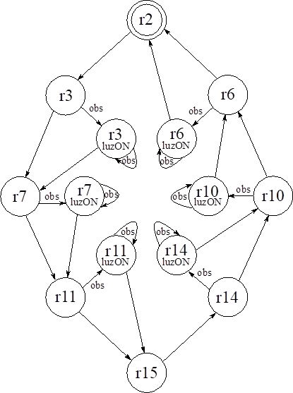
Figure 3: Automaton solution for a robot that interacts with the environment
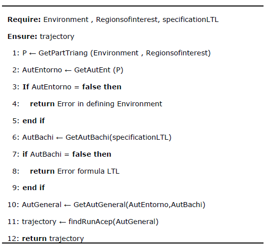
Algorithm 1: Continuous synthesis of control policies for case 1
The function that calculates the next state requires, as an input argument, to know the present state of the path in which the robot is located, as well as the census information to execute the actions defined in case any obstacles come across (stay at the same point until the obstacle disappears, recalculate the route avoiding the obstacle, generate an alert).
Case 2 - multiple robots and fixed obstacles
For the case of a team of identical robots modeled, which move in a rectangular environment, initially, it can be assumed that, with an adaptation of Algorithm 1, the problem can be solved. However, the need for synchronization between the automatons of each of the robots make the automaton in the environment grow in a way | P | ^ n * | B |, where | P | is the number of partitions present in the workspace, n is the number of robots, and | B | is the number of states in the Büchi automaton. This implies that, as the number of robots increases, the consumption of resources for processing increases, until a point is reached where there is a combinational explosion of states. A methodology is then proposed which involves the use of Petri nets to describe the workspace. A finite set of atomic sentences is assumed Π = π_1, π_2,…, π_ | Π |, where π_i labels a specific region of interest that corresponds to one or more cells in the environment, and, if at least one robot is in any of these cells, the π_i proposition is said to be true (True).
The set Π is used to provide an LTL formula that defines the task to be accomplished by the robot team. The initial marking of the network system is m_0 = [1,0,0,0,1] ^ T, the output alphabet is Π = π_1, π_2, π_3, π_4, π_5, and the observation map: h (a_1) = π_1, h (a_2) = π_2, h (a_3) = π_3, h (a_4) = π_4, and h (a_5) = π_5. The characteristic vector of π_i is v_i = [p_0, p_1,…, p_n], with n being the number of cells into which the workspace is divided and p_i = 1 if and only if π_i is observable in a_i. With the previous vectors the transition matrix is constructed
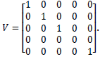 .
.
Since V ∙ m_0 = [1,0,0,1] ^ T, observations π_1 and π_5 are active at m_0 because the initial location of the robots is a_1 and a_5. An execution (or trajectory) of Q is a finite sequence r = m_0 [├ t_j1⟩ m_1 [├ t_j2⟩ m_2 [├ t_j3… t_ (j_ | r |) ⟩m_ | r |, which produces an output word, which is the observed sequence of 2 ^ Π elements, and LTL formulas are interpreted over infinite chains of observations from 2Π (Clarke et al., 1999). As in this case, only the co-safe LTL formulas are considered. Any LTL formula on the set Π can be transformed into a Büchi automaton, which accepts only the input strings that satisfy the formula (Wolper et al., 1983). Some available software tools that allow such conversions are described in the literature (Gastin & Oddoux, 2001; Holzmann, 2003). Considering that the activation specifications for the RdP are generated based on a requirement given as a Boolean formula, a finite set of atomic sentences is defined Π = {Π_1, Π_2, Π_3,…, Π_ | π | }, where the Π_i tags represent a specific region of interest in the environment. The requirements are expressed as a Boolean logical formula on the set of variables P = P_t∪P_f, where P_t = Π and P_f = {π_1, π_2,…, π_ | Π | }. The sets P_t and P_f refer to the same regions of interest, but the elements of P_t indicate the regions that must be visited throughout the execution of the trajectory, and the elements of P_f indicate the regions that must be visited in the last execution status. The specifications are interpreted as finite words over the set 2 ^ Π.
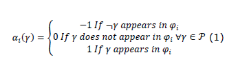
In general, the composition of set P is evaluated on the word generated by the execution r = m_0 [├ t_j1⟩ m_1 [├ t_j2⟩ m_2 [├ t_j3… t_ (j_ | r |)⟩ m_ | r | considering the following conditions: i) Π_i∈P_t is true when evaluating it on the word h (r) if and only if ∃j∈ {0,1,…, | r |} such that Π_i∈ || V ∙ m_j ||; ii) Π_i∈P_f is true when evaluating it on the word h (r) if and only if Π_i∈ || V ∙ m_j ||. Furthermore, all Boolean-based φ requirements must be expressed in Conjunctive Normal Form (FNC), and such requirements represent the task that the entire robot team must fulfill and do not specify the functions of each robot at an individual level. All logical expressions can be expressed in FNC (Brown, 2012), and, when expressing φ in FNC, we have a conjunction of n terms φ = φ_1∧φ_2∧… ∧φ_n. Each of the terms φ_i | i = 1,2,…, n are a disjunction of n_i variables of set P with the form [π_2│¬π_2] ∨… ∨ [Π_ (jn_t) │¬Π_ (jn_t)] ∨ [π_ (jn_t) | ¬π_ (jn_t)]. As any Boolean formula in FNC form can be converted to a set of linear inequalities using various techniques (Smaus, 2007), a binary vector x = [x_ (Π_1), x_ (Π_2),…, x_ (Π_ | Π |), x_ (π_1), x_ (π_2),…, x_ (π_ | Π |)] ^ T∈ {0,1} ^ (2 ∙ Π) with 2 ∙ Π variables evaluating for each component of the vector the following conditions: i) x_ (Π_i) = 1 if the proposition Π_i is evaluated true, that is, if the region labeled Π_i is visited at any time during the execution of the trajectory and x_ (Π_i) = 0 if the region tagged as Π_i is NOT visited. ii) x_ (π_i) = 1 if the proposition π_i evaluates to be true, that is, if a robot stops within the region labeled π_i and x_ (π_i) = 0 if a robot does NOT stop within the labeled region as π_i, ∀i = 1,2,…, | Π |. Based on the previous conditions, it is defined that φ is equivalent to a set of n linear inequalities, where each corresponds to a disjunctive term φ_i, i = 1,…, n. To formally construct these inequalities, for each φ_i, a function α_i ∶P → {-1,0,1} is defined which shows which variables of P appear in the disjunction φ_i and which of these are negated.
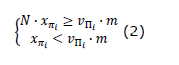
Formally, the linear inequality corresponding to the disjunction φ_i is given by Σ γ∈P (α_i (γ)∙x_γ)≥1++Σγ∈Pmin (αi (γ),0), where min(αi (γ),0) is the minimum value between α_i and 0. Equations (1) and (2) start from the following assumptions: if the region corresponding to the symbol γ∈P is not visited according to φ_i, then its corresponding binary variable has a coefficient α_i (γ) = 0. Out of all the regions that appear as not negated in the disjunction φ_i, at least one must be visited, and, therefore, the sum of all its corresponding binary variables must be greater than or equal to 1. A negated symbol γ means the avoidance of a region, either along a path or in the final state, which implies that its corresponding binary variable x_γ must be zero. In this way, a specification of the FNC form is algorithmically convertible, through Equation (2), into a system of n linear inequalities, one for each disjunctive term. For each of the observations of Π_i, a binary variable x_ (π_i) = 1 is set if π_i is evaluated as true in a final state of execution. In Equation (2), a set of linear inequalities is proposed which can be used to define the value of the binary variable x_ (π_i) in a final marking m, where N is the number of robots and v Π i is the vector characteristic of observations of πi.
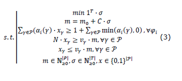
When finding a solution for the proposed problem, the goal is to minimize the number of transitions along the path. Therefore, the cost function 1 ^ T ∙ σ is chosen, and the MILP problem is formulated in Equation (3) to obtain a final markup in which the specification is met, where v_γ is the characteristic vector of γ∈P. The solution is obtained by activating the enabled transitions and storing the sequence of places visited by each brand.
To include compliance with the constraints on the trajectory, a sequence of k marks m_1, m_2,…, m_k is considered so that m_1 = m_0 + C ∙ σ_1, m_0-Pre ∙ σ_1≥0; m_2 = m_1 + C ∙ σ_2, m_1-Pre ∙ σ_2≥0… This implies that, between the states of the RdP m_ (i-1) and m_i, each mark moves at most through one transition, and thus the triggering of transitions for empty places is avoided.
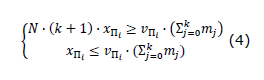
For each of the specifications Π_i that belong to the path constraint, a binary variable Πi = 1 is introduced as long as it is evaluated as true along the path y. As the path is given by the sequence of the k intermediate marks, Equation (4) is defined as the set of linear inequalities that consider all intermediate marks and not only the final mark as in Equation (3).
Finally, the solution to this case involves choosing a sequence of observations that satisfies the LTL formula and then generating the appropriate sequence of activations in NMR that produce that sequence. This solution is based on three main steps: i) a good finite prefix r (called run) is chosen from the Büchi automaton which corresponds to the LTL formula; ii) for each transition of run r, a sequence of activations is searched for the NMR model so that the observations generated produce the chosen transition; iii) the movement strategies of the robots are obtained by concatenating the firing sequences of step 2 and imposing synchronization moments between them.
Step i: to find a set of paths from B, for example, using a k-shortest path algorithm (Yen, 1971) on the adjacency plot corresponding to the transitions of B.
Step ii: to enable the transition s_j → s_ (j + 1) in B, j = 0,…, L_r-1, the following two conditions must be valid: a) the RMPN system must reach a final mark m that generates any observation of the set ρ (s_j, s_ (j + 1)) ⊆2 ^ Π; b) intermediate NMRN marks must generate only observations in the set ρ (s_j, s_j) ⊆2 ^ Π, so that s_j is not left in states other than s_ (j + 1). To verify an observation at a given achievable mark m, for each observation π_i∈Π, a binary variable x_i is defined in such a way that: x_i = 1, IF v_i ∙ m> 0, and x_i = 0 if otherwise. The following two conditions assign the correct value to x_i:
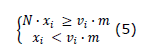
It is highlighted that, if v_i ∙ m> 0, the first restriction of Equation (5) is x_i = 1, while the second restriction ensures that x_i = 0 if v_i ∙ m = 0.
Require: Environment, Regionsofinterest, specificationLTL, CPLEX
Ensure: sequence [sequence of activations per robot]
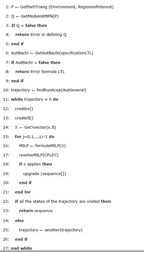
Algorithm 2: Continuous synthesis of control policies for case 2
Step iii: To derive appropriate formal descriptions equivalent to the conditions expressed in Equations (4) and (5), a generic subset S⊆2 ^ Π is considered. It is desired that the set of active observations in a mark m is included in S. The set S can be seen as a disjunction of conjunctions of propositions of Π to convert it into a Conjunctive Normal Form (FNC) by double negation, that is, the observations in m should not belong to 2Π / S. By already having the FNC set, it can be used to write a set of inequalities that hold simultaneously so that the observations in m belong to S (Martínez et al., 2018).
Steps ii and iii must be iterated, taking, at each iteration, another run r from the constructed set of possible runs of B. Once a run can be followed due to the RMPN observations (step ii was successful), the process can be considered as concluded, and the solution returned is given by the currently chosen execution of B, that is, by r = s_0 s_1… s_ (L_r), where L_r is the length of r.
These steps are implemented through Algorithm 2, in which the CPLEX software provided by IBM is used to solve the MILP problem that arises.
EXPERIMENTS AND RESULTS
The experiment is configured for the implementation of the algorithms proposed, using the Matlab programming software installed on a Windows 7 operating system on an ASUS X555L laptop with an Intel Core i7 processor (4510U, 3.1 GHz), 8 GB RAM, and a toolbox under development proposed by the authors for robot movement that was used as support. For the problem posed above, the displacement specification is given by the LTL formula φ = ⋄a_2∧⋄a_15. The trajectory obtained when executing Algorithm 1 to solve this problem can be seen in the upper left part of Figure 4, and the respective data associated with the execution in column "Route 1" of Table 2. It should be noted that, in this case, the longest processing time is associated with the generation of the diagram of states and transitions for the robot, and that this diagram is directly linked to the number of regions into which the space is divided, as well as to the relation of adjacency between them. It can also be noted that the trajectory obtained does not evade the obstacles present in the workspace (regions 1,3, ..., 14,16), so the LTL specification cannot be considered as fulfilled. The problem is then solved through the execution of Algorithm 1, and an obstacle avoidance condition is included in the specification, such as the formula φ = ⋄a_2∧⋄a_15∧ □ ¬ (a_1∨a_3∨a_4∨ … ∨a_14∨a_16). Thus, a new set of results is obtained consisting of the path in the upper right part of Figure 4 and the column “Path 2” of Table 2. The resulting trajectory complies with the given specification since it only enters regions 2 and 15, always avoiding the other regions of interest to the system. When comparing the results of "Route 1" and "Route 2" in Table 2, a noticeable difference is identified in the time associated with the generation of the diagram of states and transitions of the robot, which directly affects the time associated with calculating acceptable routes that meet the specification. This indicates that the more robust the LTL formula in terms of delimiting the behavior of the workspace, the less time it takes to calculate a solution path. The possibility of including more robust LTL formulas implies the possibility of executing different types of tasks in the same environment, which is subject to the same complexity in the generation of the robot's transition system. Talking about various types of tasks directly refers to the possibilities of expression of logical tasks that the LTL formulas provide, mainly, security, coverage, or sequencing. The trajectory in the upper right part of Figure 4 refers to a co-safe specification and corresponds to the trajectory with the fewest number of transitions in the automaton of the complete system. However, if more regions of interest are included, this will remain the only criterion, that is, the system delivers the shortest route that covers the three regions, regardless of the order in which it covers them. An example of the above is the case of the route shown in the lower left part of Figure 4 and column “Route 3” of the Table 2, which expresses the trajectory and the resulting data for the LTL formula φ = ⋄a_2∧⋄a_15∧⋄a_12∧ □ ¬ (a_1∨a_3∨a_4∨… ∨a_11∨a_13∨a_14∨a_16), which in turn includes region 12 as a region of interest.
Source: Authors
Table 2: Data resulting from Algorithm 1 in the calculation of the trajectories of Figure 4
Criterion
Path 1
Path 2
Path 3
Path 4
Transition system for a single robot (states)
130
130
130
130
Time to generate diagram (seconds)
2,328
0,247
0,201
0,146
Buchi automaton for solution LTL (states)
4
4
8
6
Complete system automation (states)
520
520
1040
780
Time to generate complete system automation (seconds)
0,157
0,062
0,167
0,114
Time to find an acceptable path in automation (seconds)
0,395
0,156
0,390
0,334
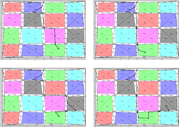
Figure 4: Trajectories obtained with Algorithm 1
However, the order in which the regions are reached is not specified, and the new expressiveness of Algorithm 1 makes it possible to do so by changing the coverage structure of the LTL formula to a sequencing structure, leaving the formula as φ=⋄(a2∧⋄(a15∧⋄(a12∧(¬a12 )Ua15 )))∧□¬(a1∨a3∨a4∨…∨a11∨a13∨a14∨a16). This last LTL formula expresses, in addition to the need to reach regions 2, 15, and 12 at some time in the future, the need to reach them in that order. The trajectory and the data corresponding to the solution found through Algorithm 1 in Matlab can be seen in the lower right part of Figure 4 and in the column “Path 4” of Table 2. To demonstrate that, in Algorithm 2, the time to find the solution does not depend on the number of robots that are added to the system, an environment with six regions of interest is proposed, and the results are obtained for two, three, four, and five robots cooperatively reaching the specification φ = A∧B∧C∧D. The formula delivered in FNC form expresses that the robot team must jointly reach the regions A, B, C, D, corresponding to the red, violet, green, and blue regions in the workspace of the Figure 5.
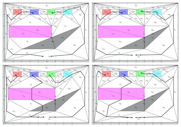
Figure 5: Trajectories obtained with Algorithm 2
It is evident that the specification is met in all cases. However, it is also noted that not in all cases do all the robots move. That is, in some cases, a few robots move to reach the specification while the others remain static. This is because the algorithm is optimal from the point of view of the number of transitions that must be activated to reach the specification, which implies, in this case, that moving all the robots generates more shots in the transitions than they are needed. Table 3 shows the compilation of the data obtained for each of the algorithm executions in the calculation of the trajectories deposited in Figure 5. In this case, the rows represent the measurement criteria, where P represents the size of places that the resulting RdP contains; T represents the number of transitions of the RdP; tp represents the time it takes the system to build the RdP; VMILP represents the number of variables that are generated for the MILP problem; = represents the number of equality restrictions; ≠ represents the number of inequality restrictions; tc(MILP) represents the time needed to build the MILP problem; Tr(MILP) represents the time required to solve the MILP problem; and, TR1,TR2,TR3,TR4, and TR5 represent the sets of activations corresponding to the trajectories of each robot
Source: Authors
Table 3: Resulting data for the calculation of trajectories in Figure 5
Criterion
2 robots
3 robots
4 robots
5 robots
𝑃
52
52
52
52
𝑇
152
152
152
152
𝑇p
0,287
0,306
0,296
0,298
VMILP
2053
2053
2053
2053
=
520
520
520
520
≠
600
600
600
600
𝑡𝑐(𝑀𝐼𝐿𝑃)
0,287
0,306
0,296
0,298
𝑇𝑟(𝑀𝐼𝐿𝑃)
0,265
0,185
0,252
0,248
𝑇𝑅1
47, 8, 11, 9, 14, 2, 16, 1, 15, 17, 23
47, 8, 11, 14, 9, 2, 15, 17, 24, 18, 20
47, 8, 11, 9, 14, 2, 16, 17
47, 7, 8, 14, 9, 2, 1, 17
𝑇𝑅2
47, 46, 7, 45, 37, 35, 38, 36, 39, 40
47, 46, 7, 45, 43, 41, 38, 42, 39, 40
47, 8, 49, 4, 13, 32, 5, 51, 24
47, 7, 8, 24, 13, 50, 4, 52, 18
𝑇𝑅3
47
47, 46, 7, 45, 37, 41, 36, 34, 22, 28
47, 46, 5, 45, 43, 41, 42, 39, 40
𝑇𝑅4
47
47
𝑇𝑅5
47
CONCLUSIONS
The proposed methodology solves the problem of synthesis of automata for the high-level control of agents (robots), where the planning of movements or the change of tasks during execution is a constant.
It was shown that, with the proposed method to change the global task of a robot team, it is only necessary to change the task given as an LTL or FNC formula.
It was also shown that, under certain criteria, the combinational state explosion problem associated with multi-agent systems can be mitigated.
It was demonstrated that many complex behaviors of robotic systems can be expressed in temporal logic, and therefore their solution can be calculated using the proposed methodology.
The presented method automatically schedules the tasks to be executed by a team of cooperating mobile robots to achieve a given task as a co-secure LTL formula or a Boolean formula in FNC form.
The solution found is optimal with regard to the number of transitions followed by the team members.
Acknowledgements
ACKNOWLEDGEMENTS
The authors would like to thank the support of Universidad Tecnológica de Pereira, its Electrical Engineering and Master’s in Electrical Engineering programs, and the Research Group for the Management of Electrical, Electronic, and Automatic Systems.
REFERENCES
FUNDING
This scientific research article is derived from the research project “A methodology for estimating the irrigation status of crops in a wide area based on NDVI and deep learning” financed by Universidad Tecnológica de Pereira (starting year: 2019; end year: 2020).
Licencia
Esta licencia permite a otros remezclar, adaptar y desarrollar su trabajo incluso con fines comerciales, siempre que le den crédito y concedan licencias para sus nuevas creaciones bajo los mismos términos. Esta licencia a menudo se compara con las licencias de software libre y de código abierto “copyleft”. Todos los trabajos nuevos basados en el tuyo tendrán la misma licencia, por lo que cualquier derivado también permitirá el uso comercial. Esta es la licencia utilizada por Wikipedia y se recomienda para materiales que se beneficiarían al incorporar contenido de Wikipedia y proyectos con licencias similares.