DOI:
https://doi.org/10.14483/udistrital.jour.reving.2017.2.a05Published:
2017-05-05Issue:
Vol. 22 No. 2 (2017): May - AugustSection:
Special Section: Best Extended Articles - WEA 2016Assessment of Effects of a Delay Block and a Nonlinear Block in Systems with Chaotic Behavior Using Lyapunov Exponents
Evaluación del Efecto de un Retardo y una No Linealidad en Sistemas con Comportamiento Caótico Utilizando Exponentes de Lyapunov
Keywords:
Chaos, Dynamical Systems, Lyapunov Exponents, Nonlinear Characteristic. (en).Keywords:
Caos, Característica No lineal, Exponentes Lyapunov, Sistemas Dinámicos (es).Downloads
References
Kathleen T Alligood, Tim Sauer, and James A Yorke. Chaos: an introduction to dynamical systems. New York;[London]: Springer, 2011.
John Guckenheimer and Philip J Holmes. Nonlinear oscillations, dynamical systems, and bifurcations of vector fields, volume 42. Springer Science & Business Media, 2002.
RW Brockett. ”On conditions leading to chaos in feedback systems”. In Decision and Control, 1982 21st IEEE Conference on, pages 932–936. IEEE, 1982.
R Genesio and A Tesi. ”Chaos prediction in nonlinear feedback systems”. In IEE Proceedings D-Control Theory and Applications, volume 138, pages 313–320. IET, 1991.
Arturo Buscarino, Luigi Fortuna, Mattia Frasca, G Sciuto, and MG Xibilia. ”Harmonic balance method for time–delay chaotic systems design”. In IFAC Proceedings Volumes, volume 44, pages 5112–5117. Elsevier,2011.
AC Barrag´an and JJ Soriano. ”Describing function based analysis of the characteristics of chaotic behavior in the jerk dynamic system”. Central America and Panama Convention (CONCAPAN XXXIV), 2014 IEEE, pages 1–6, 2014.
Thomas J¨ungling and Wolfgang Kinzel. ”Scaling of Lyapunov exponents in chaotic delay systems”. arXiv preprint arXiv:1210.3528, 2012.
Hongyan Jia, Qinghe Wang, Qian Tao, and Wei Xue. ”Analysis and Circuit Implementation for the Fractional-order Chen System”. In 8th CHAOS Conference proceedings, 2016.
Benjamin C Kuo. Sistemas de control autom´atico. Pearson Educaci´on, 1996.
M Vajta. ”Some remarks on Pad´e-approximations”. In Proceedings of the 3rd TEMPUS-INTCOM Symposium,
Halsey Lawrence Royden and Patrick Fitzpatrick. Real analysis, volume 198. Macmillan New York, 1988.
Steven H Strogatz. Nonlinear dynamics and chaos: with applications to physics, biology, chemistry, and
engineering. Westview press, 2014.
Witold Kinsner. ”Characterizing chaos through Lyapunov metrics”. IEEE Transactions on Systems, Man, and
Cybernetics, Part C (Applications and Reviews), 36(2):141–151, 2006.
Melke A Nascimento, Jason AC Gallas, and Hamilton Varela. ”Self-organized distribution of periodicity and chaos in an electrochemical oscillator”. Physical Chemistry Chemical Physics, 13(2):441–446, 2011.
Laura M Perez, Jean Bragard, Hector Mancini, Jason AC Gallas, Ana M Cabanas, Omar J Suarez, and David Laroze. ”Effect of anisotropies on the magnetization dynamics”. Networks and Heterogeneous Media, 10(1):209–221, 2015.
Marco Sandri. ”Numerical calculation of Lyapunov exponents”. Mathematica Journal, 6(3):78–84, 1996.
K Ramasubramanian and MS Sriram. ”A comparative study of computation of Lyapunov spectra with different algorithms”. Physica D: Nonlinear Phenomena, 139(1):72–86, 2000.
How to Cite
APA
ACM
ACS
ABNT
Chicago
Harvard
IEEE
MLA
Turabian
Vancouver
Download Citation
Evaluación del Efecto de un Retardo y una No Linealidad en Sistemas con Comportamiento Caótico Utilizando Exponentes de Lyapunov
Assessment of Effects of a Delay Block and a Nonlinear Block in Systems with Chaotic Behavior Using Lyapunov Exponents
Pablo Rodríguez Gómez
Universidad Distrital Francisco José de Caldas. Bogotá - Colombia,
pcrodriguezg@correo.udistrital.edu.co
Maikoll Rodríguez Nieto
Universidad Distrital Francisco José de Caldas. Bogotá - Colombia,
marodriguezn@correo.udistrital.edu.co
Jairo Soriano Mendez
Universidad Distrital Francisco José de Caldas. Bogotá - Colombia,
jairosoriano@udistrital.edu.co
Received: 20/12/2016. Modified: 10/03/2017. Accepted: 31/03/2017.
Abstract
Context: Because feedback systems are very common and widely used, studies of the structural characteristics under which chaotic behavior is generated have been developed. These can be separated into a nonlinear system and a linear system at least of the third order. Methods such as the descriptive function have been used for analysis.
Method: A feedback system is proposed comprising a linear system, a nonlinear system and a delay block, in order to assess his behavior using Lyapunov exponents. It is evaluated with three different linear systems, different delay values and different values for parameters of nonlinear characteristic, aiming to reach chaotic behavior.
Results: One hundred experiments were carried out for each of the three linear systems, by changing the value of some parameters, assessing their influence on the dynamics of the system. Contour plots that relate these parameters to the Largest Lyapunov exponent were obtained and analyzed.
Conclusions: In spite non-linearity is a condition for the existence of chaos, this does not imply that any nonlinear characteristic generates a chaotic system, it is reflected by the contour plots showing the transitions between chaotic and no chaotic behavior of the feedback system.
Keywords: Chaos, Dynamical Systems, Lyapunov Exponents, Nonlinear Characteristic.
Language: English
Resumen
Contexto:Al ser los sistemas realimentados muy comunes y ampliamente usados, se han desarrollado estudios de las características estructurales bajo las cuales se genera comportamiento caótico. Estos pueden ser separados en un sistema no lineal y un sistema lineal por lo menos de tercer orden. Se han usado métodos como la función descriptiva para su análisis.
Método:Se propone un sistema realimentado a partir de un sistema lineal, un sistema no lineal y un retardo, con el fin de evaluar su comportamiento utilizando los exponentes de Lyapunov. Se evalúa con tres diferentes sistemas lineales, diferentes valores del retardo y diferentes valores para los parámetros de una característica no lineal, buscando alcanzar un comportamiento caótico.
Resultados: Se realizaron cien experimentos para cada uno de los tres sistemas cambiando el valor de algunos parámetros evaluando la influencia de los mismos en la dinámica del sistema. Se realizan y analizan gráficas de contorno que relacionan estos parámetros con el máximo exponente de Lyapunov.
Conclusiones: A pesar que la no linealidad es una condición para que exista caos, esto no implica que cualquier característica no lineal genera un sistema caótico, esto se evidencia en las gráficas de contorno mostrando las transiciones entre comportamiento caótico y no caótico del sistema realimentado.
Palabras clave: Caos, Característica No lineal, Exponentes Lyapunov, Sistemas Dinámicos.
Idioma: Inglés
1. Introducción
The chaos has been object of study since past century and it has generated more interest in the researchers since was discovered that in nature exist systems with this type of behavior [1]. The chaotic systems also have been object of study in the control area due to they can be analyzed with mathematical tools of dynamical systems [2]. In practice is common to see systems which exhibit pure delays, either by their nature or by the controller used, anyway the system behavior is affected. One particular case are the systems with negative feedback which exhibit chaotic behavior under specific structural conditions. In [3], [4] feedback systems are shown which exhibit this behavior, also a structure is shown which divides the systems into a linear block and a nonlinear block in order to facilitate the analysis. It enlarges the study scope to search structural conditions and pure delay effects which generate chaotic behavior, which can be evaluated via different methods. For example, in [4]-[6] an evaluation is made by the descriptive function method. In [7], dynamical systems with time-delayed feedback are studied using Lyapunov exponents to identify strong or weak chaos. In [8], a numerical analysis of chaotic behavior of fractional-order Chen system is performed, using Lyapunov exponents and bifurcations diagrams.
In this work the chaotic behavior of a feedback system proposed is evaluated using Lyapunov exponents and phase plane. This system is composed of a linear block, a nonlinear block and a delay. Three linear systems are proposed, a pure delay which is implemented in simulation using the Transport Delay Simulink block and the non-linearity is built. In contrast to works [7], [8], the initial point is not a known chaotic system. In this case, the chaotic system is designed, built and assessed in order to identify which values of parameters are most influentials to chaotic behavior. This paper is organized as follows: In sections 2, 3 and 4 is described the conceptual framework for develop the study, in section 5 the proposed feedback system and its elements are described in greater detail, in section 6 is showed how the simulation was implemented and the outcomes obtained for each evaluated case, and in section 7 the conclusions obtained are described.
2. Delay Systems
A continuous system is the one in which the continuous input signals are transformed into continuous output signals. A system can present an inherent delay that causes a time-shift in the input signal but does not affect his characteristics, this kind of delay is called pure delay. In practice is possible to find pure delays in some kind of systems, especially those with hydraulic, pneumatic or mechanical transmissions. The computer control systems also have delays as they require some time to perform numerical operations [9].
2.1. Padé Approximation
The pure delay transfer function is e L S, which Padé approximation is a rational function (1), where Pm(s) is a polynomial defined by (2) and Qn(s) is a polynomial defined by (3) where n and m represent the degree of each polynomial [10]. The roots of polynomial Pm(s) are called zeros and the roots of polynomial Qn(s) are called poles [9].
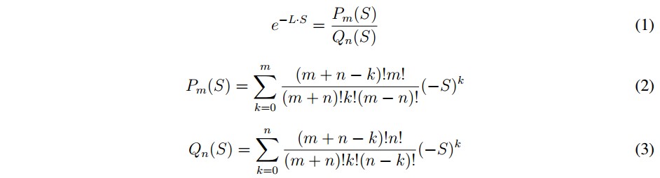
Is possible to choose n = m to add the same number of poles and zeros. This approximation is used to know what order generates a similar behavior to feedback system with delay.
3. Simple Function
A simple function is a function that satisfies φ=A ⊆ ℝ → ℝ which is given by:
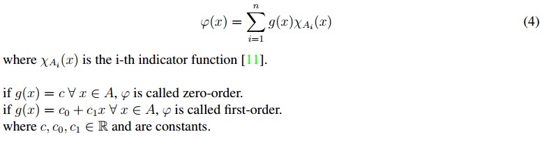
Below the simple function of first-order is used. This function is given by (5), which is used because of the ease to change the simulation parameters.

4. An Approach to Chaos in Dynamical Systems
A universally accepted definition for chaos does not exist yet, but almost every authors agree in three main features [12]:
- Aperiodic long-term behavior: There are trajectories which do not settle down to fixed points, periodic orbits, or quasiperiodic orbits in the course of time.
- Deterministic: The irregular behavior arises from the non-linearity of the system, rather than from noisy driving forces.
- Sensitive dependence on initial conditions: Two different initial conditions but nearby each other, generate different trajectories.
- Chaos can appear in feedback systems and a way to assess his behavior is through of Lyapunov exponents.
4.1. Feedback Systems
Due to the frequent use of feedback systems and all tools that exist for its analysis, it has been studied under which structural conditions a chaotic behavior is presented.
In [4] is suggested that a feedback system presents a chaotic behavior when a predicted limit cycle (PLC) and an equilibrium point (EP) of certain characteristics interact between themselves.
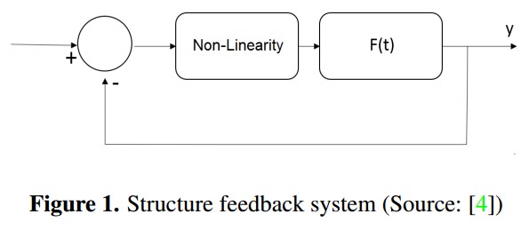
For chaos to be presented must exist a non-linearity in the system, therefore the feedback system can be represented as a linear subsystem and a nonlinear subsystem, also the lineal subsystem must be at least third order (Figure 1).
4.2. Lyapunov Exponents
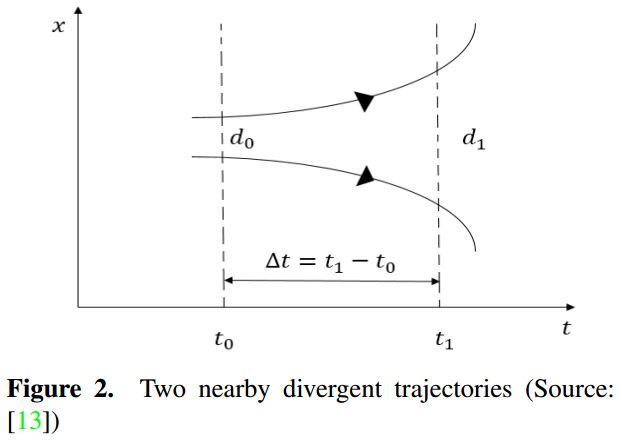
Two trajectories are considered which are separated by an initial distance d0 at time t0 that present a growth of distance (dt) between them, which is calculated by (6) over a time period ∆t [13], as illustrated in Figure 2.


The number λ is called Lyapunov exponent, is defined by (7) and is used to quantify the chaotic behavior in dynamical systems. The authors in [14], [15], use Lyapunov exponents to study the behavior of a prototype electrochemical oscillator and the magnetic anisotropy effects in a magnetic particle respectively.
Depending on the value of the Lyapunov exponent there are three options:
- λ<0, implies contraction, it means that the system converges to a fixed point.
- λ=0, the system tends to a limit cycle.
- λ>0, implies distance growth between the trajectories, the system presents chaotic behavior.
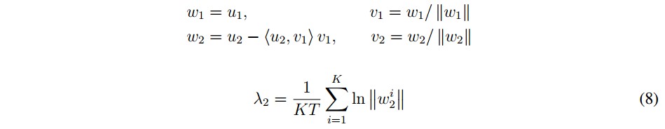
There are different methods to calculate the Lyapunov exponents as shown in [16], [17]. In the realized tests of this work the Gram-Schmidt method is used with a time span of 100 units time and 0.01 units time of transient time to three second order systems with delay. This method uses orthonormal initial conditions, e.g. u1 = [1, 0, 0, ...], u2 = [0, 1, 0, ...], ... .Variables w1, v1 y w2 are calculated; Then, using w2 value and equation 8 the Largest Lyapunov exponent is obtained, where K is the number of samples and T is the sample period.
5. System Description
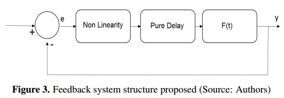
In practice, pure delays are presented in several kinds of systems [9], for this reason, a study is performed to observe whether chaotic behavior is generated from a linear system with delay and a non-linearity. One feedback system was built with these elements, as can see in Figure (3).
To perform the study, a linear system and a non-linearity were proposed following the structure suggested in [4] (Figure 1), the difference is in linear system by second order with delay and the non-linearity is built. Below explain with detail each part of the proposal.
5.1. Linear System
As is proposed in [4], a dynamical system is chaotic if his linear part is a oscillatory system and exist some feedback control features which make that system to present at least a predictable limit cycle. According to the above, three linear systems are proposed to analyze several cases or scenarios.
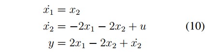
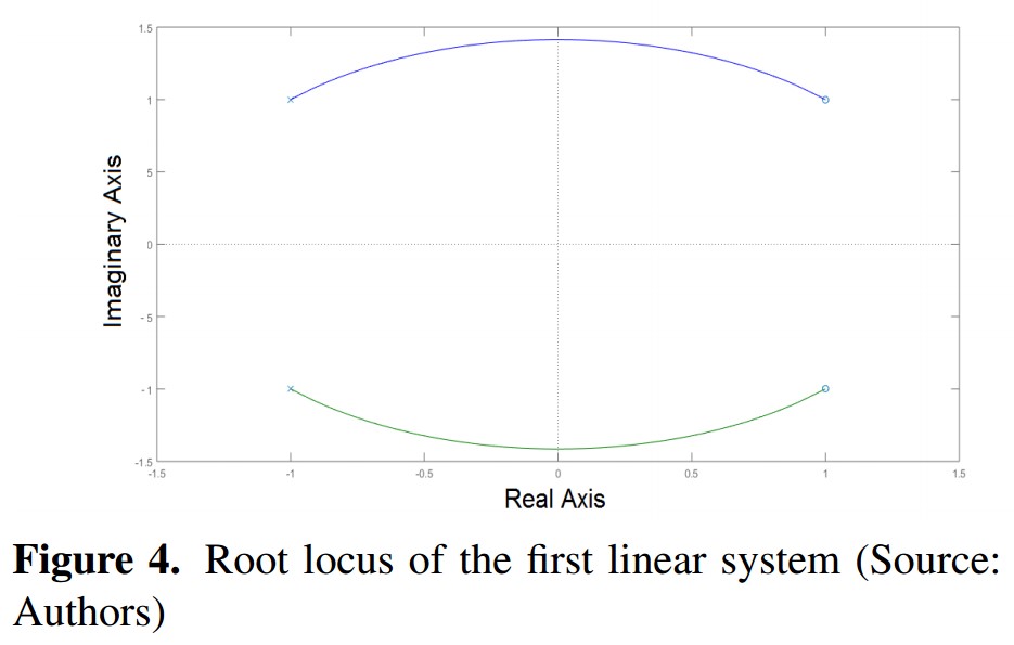
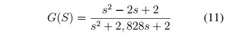
First System: It has a couple of complex conjugated poles with negative real part and two complex conjugate zeros with positive real part, which are symmetrical respect to imaginary axis. In Figure 4, is shown the root locus with the characteristics described.
The system transfer function is
The state variables representation is
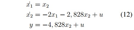
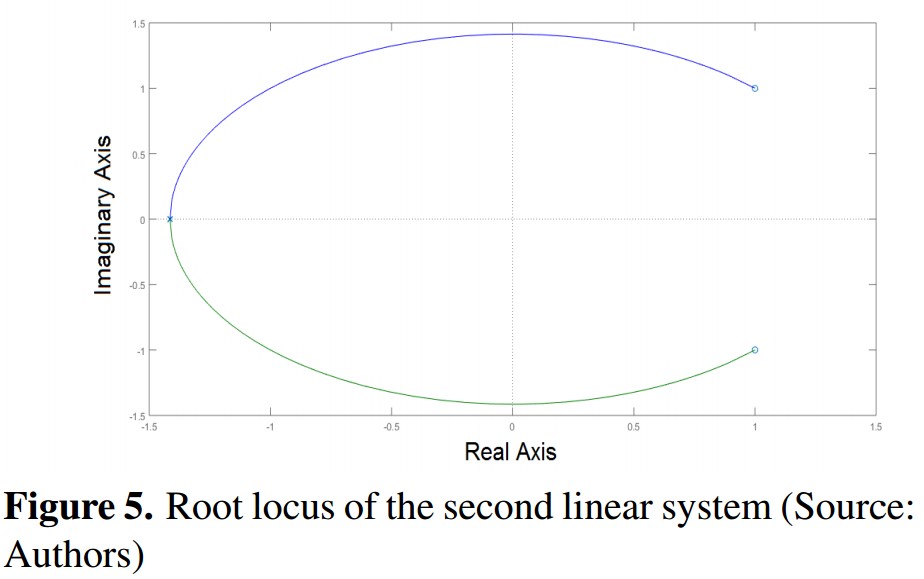
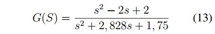
Second System: : It has a couple of complex conjugated zeros with positive real part and two real negative repeated poles. In Figure 5is shown the root locus with the characteristics described.
The system transfer function is
The state variables representation is
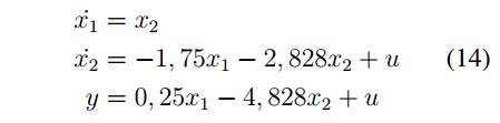
Third System: It has a couple of complex conjugated zeros with positive real part and two real negative different poles. In Figure 6 is shown the root locus with the characteristics described.
The system transfer function is
The state variables representation is
5.2. Nonlinear Block
For this particular case, the nonlinear characteristic is not inherent to the system, so it is proposed a nonlinear block built from linear functions piecewise, and is implemented using the first order simple function defined by (5).
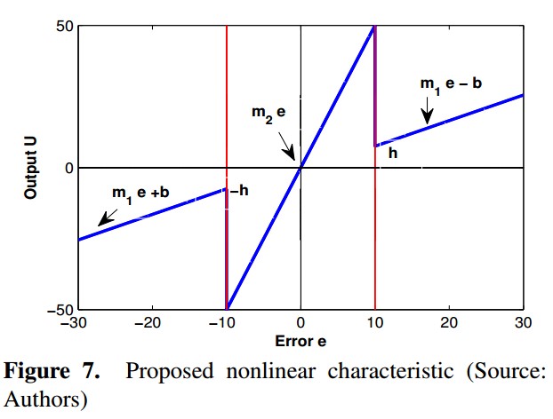
The nonlinear characteristic built is defined by (15)and is shown in Figure 7. The variable e is the input and represents the system error, defined by e = -y being "y" the feedback system output; the variable u is the output of the nonlinear characteristic and represents the input to the linear system with delay.
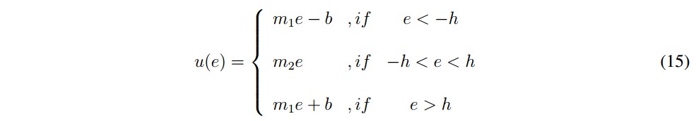
In Figure 7 the parameters that constitute the nonlinear characteristic are indicated. These Parameters are:
- m1: Slope of linear equations of the ends
- m2: Slope of internal linear equation
- b: Vertical axis intercept of the linear equations with slope m1
- h: It represents the transition between a linear equation and other.
Some considerations taken in order to select each parameter are the following. First of all, based on root locus of each linear system, the gain value where the systems are marginally stable was found and is called km, for each system the value was km = 1. Based on this gain, the parameters m1 y m2 were selected.
The gain value m2 must be greater than km to move the poles to the unstable region and the gain value m1 must be less than km to bring back the poles toward the stable region. When the error is into the m2 zone, the system becomes unstable and the error value increases until it reaches the m1 zone where the system becomes stable. These gain changes make the system have a erratic behavior and therefore, uncertainty of new values that can take the error is generated and it opens the possibility of a chaotic behavior in the system. Values of m1 and m2 that generate stronger changes of the poles position may exist. By last, the parameters h and b are selected arbitrarily. In the results section a tuning of all parameters described previously is made for a particular system, in order to identify what combinations generate chaotic behavior.
5.3. Delay
When a delay is analyzed with the Padé approximant described in section 2.1, the delay adds infinite poles and zeros to the linear system and it is converted in a superior order system. With this, the condition proposed in [4] is achieved, where is suggested that the linear system should be third order or greater. Different delay values were tried (since 0:5 until 7 time units) for a particular linear system in order to analyze effects in the feedback system.
6. Results
This section shows the implementation of the feedback system simulation which was proposed and described in preceding section. The parameters m1 and b are fixed and the parameters m2, h and the delay time (td) are modified in order to evaluate their effects in the behavior of three feedback systems.
6.1. Simulation
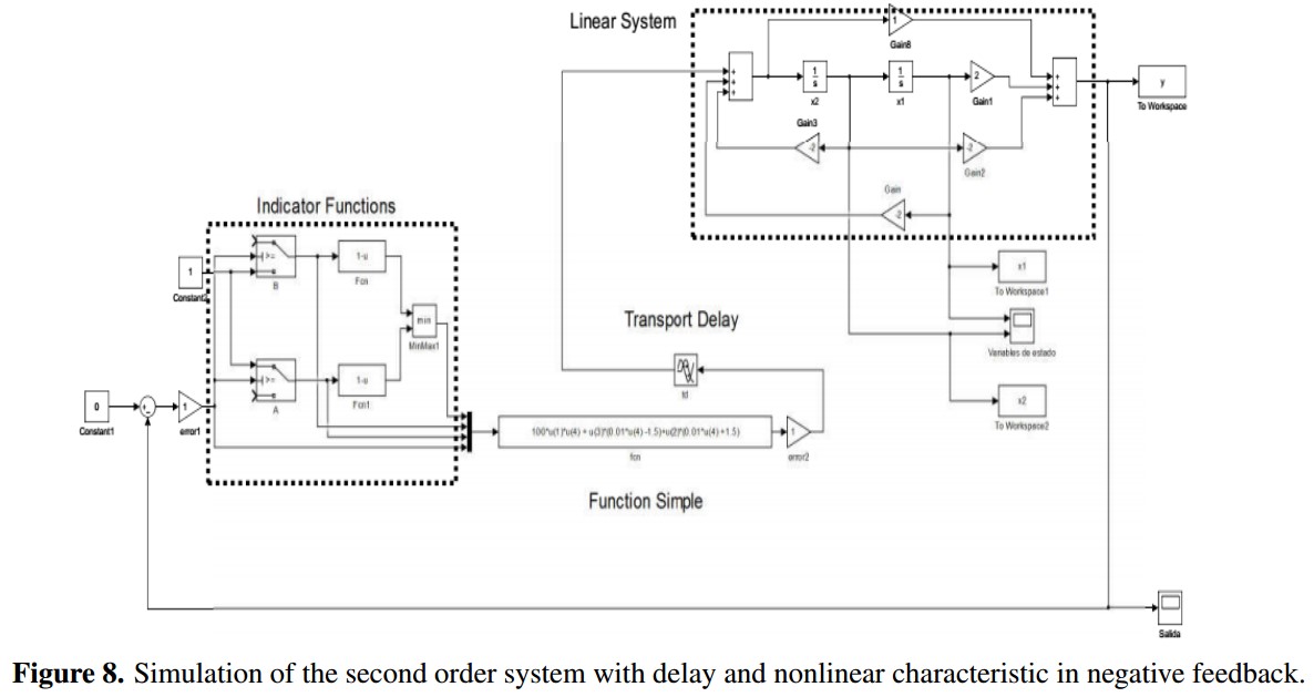
The state equations of the three linear systems are implemented (10, 12, 14). The Transport Delay Simulink block is used for set the delay, and finally for the nonlinear characteristic three indicator functions are created, one for each piece of the equation (15) and using the first order simple function defined by (5) the straight equations are implemented, this implementation is shown in Figure (8).
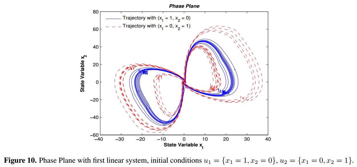
To assess the chaotic behavior of the feedback system, a copy is created with initial conditions different but very close to the original conditions and orthonormal between them (u1 = {x1= 1; x2= 0}, u2 = { x1 = 0; x2 = 1}). The data of each state variable for a time span of 100 time units are collected and exported, and the Largest Lyapunov exponents are calculated using (8) with K= 10000 and a sample period T = 0:01 time units.
6.2. Tests with Different Linear Systems
Following the considerations described in section 5, a previous study of all parameters (m1, m2, h, b y td) was made, obtaining that the parameters m2, h y td are the most influential in the feedback system behavior. In the feedback system, the linear system is changed by the three systems proposed and 100 tests are made to each one, changing the parameters values in this way: m2 between 1.1 - 101.1, h between 1 - 4 and td between 0.5 - 7. For each parameter combination, the Largest Lyapunov exponent is computed with the equation 8 and the contour plots that show how changes this exponent in function of the three parameters are showed in figures 9, 11 and 13. When the Largest Lyapunov exponent is least or equal to zero it is codified in black color and it means that there is not chaotic behavior. Also, in those figures the transitions between chaotic and no chaotic behavior are shown.
First System:
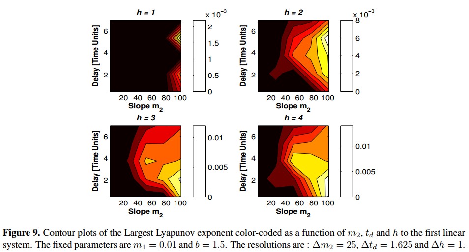
As shown in 9, as h value increases, the zone where the Largest Lyapunov exponent is positive concentrates in the lower right corner, it means td values between 0.5 and 2.125, and m2 = 101.1. The equation 8 is used to calculate the Largest Lyapunov Exponent of the 100 tests with the first linear system, and the highest was 0.01553 with h = 4, m2 = 101.1 and td = 0.5. The phase plane obtained with this values is shown in Figure 10.
Second System:
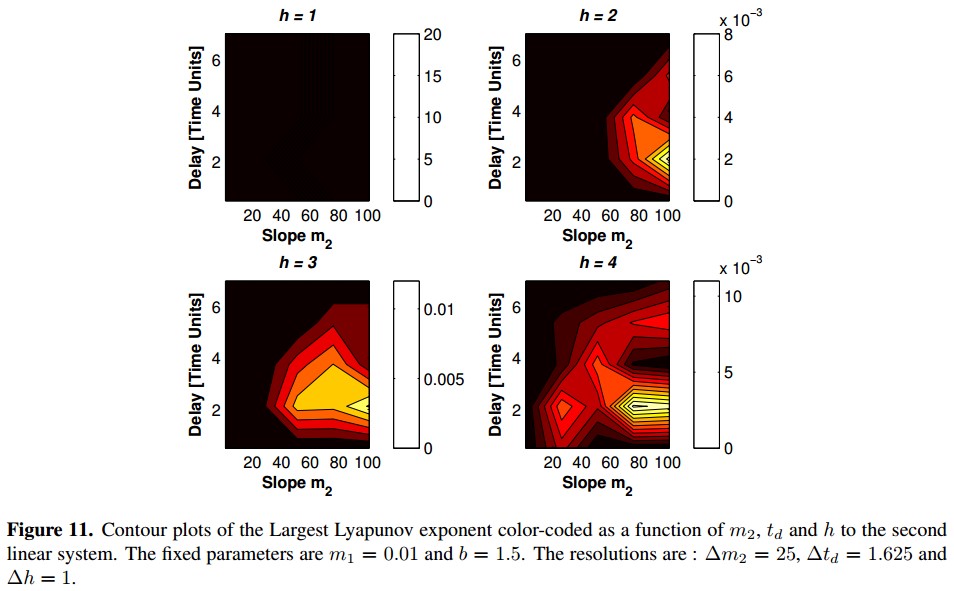
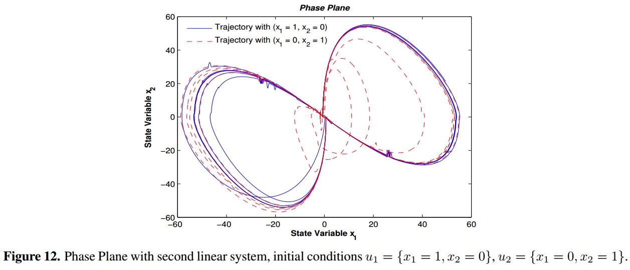
For the second linear system is highlighted that with h = 1, the system behavior is not chaotic to any combination of m2 and td, as shown in figure 11. The positive Largest Lyapunov exponent concentrates in the zone nearby to td values between 2.125 and 3.75, and m2 between 51.1 and 101.1. The equation 8 is used to calculate the Largest Lyapunov Exponent of the 100 tests with the second linear system, and the highest was 0:01124 which was obtained with h = 4, m2 = 76.1 and td = 2.125. The phase plane obtained with this values is shown in figure 12.
Third System:
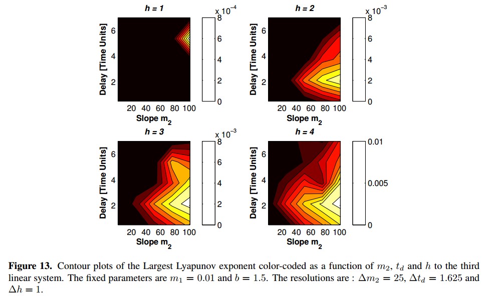
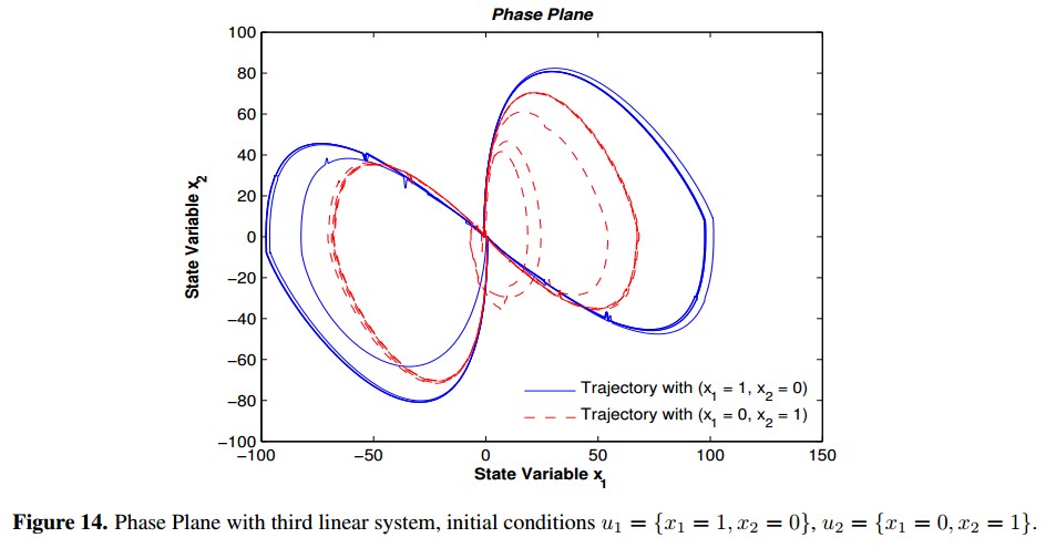
As shown in figure 13, with h = 1 the Largest Lyapunov exponent concentrates in the zone nearby to m2 = 101.1 and td = 5.375. As value of h increases, the positive Largest Lyapunov exponent concentrates in the zone of m2 = 101.1 and td values between 2.125 and 3.75. The equation 8 is used to calculate the Largest Lyapunov Exponent of the 100 tests with the third linear system, and the highest was 0.01056 which was obtained with h = 4, m2 = 101.1 and td = 2.125. The phase plane obtained with this values is shown in figure 14.
In general, changing the parameters values h, td and m2 is possible to identify the transition zones between chaotic and no chaotic behavior. As h increases, the transition point between stable and unstable regions moves away from origin (Figure 7), allowing erratic behavior be more influential in the dynamical feedback system. It is manifested numerically in the increment of Largest Lyapunov exponent. For specific h and td values, the increment of m2 manifests an increment of Largest Lyapunov exponent which represents the chaotic behavior in the system. The influence of delay value td on the Largest Lyapunov exponent in each system was particular; for the first system, the parameters td and h were the more influential while that in second and third system the more influential parameters were h and m2.
4. Conclusions
Under the considerations and the systems proposed in this paper there are certain observations.
The proposed second order systems, are more likely to have disturbances in their natural behavior due to external factors. This study allowed an assessment of the impact of a pure delay and a nonlinear block for a particular linear system, and how a built feedback system using this elements presents chaotic behavior. The tool that allowed this study was Lyapunov exponents due to they are interpretable and easy to implement when is identifying chaotic behavior in the systems.
In spite non-linearity is a condition for the existence of chaos, this does not imply that any nonlinear characteristic generates a chaotic system. Separately, delay and nonlinear characteristic make to feedback system modify its dynamic and a limit cycle is created. Together, they can generate chaotic behavior under the right conditions, such as those achieved when the parameters values were changed, watching the transitions of system dynamics between chaotic and no chaotic behavior.
This work gives rise to try out other systems with different structures, other types of non-linearity, other methods to build the non-linearity and an exploration into delay approximation with a greater order, being mindful that the chaotic behavior in the systems is being evaluated.
References
[1] Kathleen T Alligood, Tim Sauer, and James A Yorke. Chaos: an introduction to dynamical systems. New York;[London]: Springer, 2011. 241
[2] John Guckenheimer and Philip J Holmes. Nonlinear oscillations, dynamical systems, and bifurcations of vector fields, volume 42. Springer Science & Business Media, 2002. 241
[3] RW Brockett. "On conditions leading to chaos in feedback systems". In Decision and Control, 1982 21st IEEE Conference on, pages 932-936. IEEE, 1982. 241
[4] R Genesio and A Tesi. "Chaos prediction in nonlinear feedback systems". In IEE Proceedings D-Control Theory and Applications, volume 138, pages 313-320. IET, 1991. 241, 243, 244, 245, 247
[5] Arturo Buscarino, Luigi Fortuna, Mattia Frasca, G Sciuto, and MG Xibilia. "Harmonic balance method for time-delay chaotic systems design". In IFAC Proceedings Volumes, volume 44, pages 5112-5117. Elsevier, 2011. 241
[6] AC Barragán and JJ Soriano. "Describing function based analysis of the characteristics of chaotic behavior in the jerk dynamic system". Central America and Panama Convention (CONCAPAN XXXIV), 2014 IEEE, pages 1-6, 2014. 241
[7] Thomas Jungling and Wolfgang Kinzel. "Scaling of Lyapunov exponents in chaotic delay systems". arXiv preprint arXiv:1210.3528, 2012. 241
[8] Hongyan Jia, Qinghe Wang, Qian Tao, and Wei Xue. "Analysis and Circuit Implementation for the Fractional-order Chen System". In 8th CHAOS Conference proceedings, 2016. 241
[9] Benjamin C Kuo. Sistemas de control automatico. Pearson Educación, 1996. 242, 244
[10] M Vajta. "Some remarks on Padé-approximations". In Proceedings of the 3rd TEMPUS-INTCOM Symposium, 2000. 242
[11] Halsey Lawrence Royden and Patrick Fitzpatrick. Real analysis, volume 198. Macmillan New York, 1988. 242
[12] Steven H Strogatz. Nonlinear dynamics and chaos: with applications to physics, biology, chemistry, and engineering. Westview press, 2014. 243
[13] Witold Kinsner. "Characterizing chaos through Lyapunov metrics". IEEE Transactions on Systems, Man, and Cybernetics, Part C (Applications and Reviews), 36(2):141-151, 2006. 243, 244
[14] Melke A Nascimento, Jason AC Gallas, and Hamilton Varela. "Self-organized distribution of periodicity and chaos in an electrochemical oscillator". Physical Chemistry Chemical Physics, 13(2):441-446, 2011. 244
[15] Laura M Perez, Jean Bragard, Hector Mancini, Jason AC Gallas, Ana M Cabanas, Omar J Suarez, and David Laroze. "Effect of anisotropies on the magnetization dynamics". Networks and Heterogeneous Media, 10(1):209-221, 2015. 244
[16] Marco Sandri. "Numerical calculation of Lyapunov exponents". Mathematica Journal, 6(3):78-84, 1996. 244
[17] K Ramasubramanian and MS Sriram. "A comparative study of computation of Lyapunov spectra with different algorithms". Physica D: Nonlinear Phenomena, 139(1):72-86, 2000. 244
License
![]()
From the edition of the V23N3 of year 2018 forward, the Creative Commons License "Attribution-Non-Commercial - No Derivative Works " is changed to the following:
Attribution - Non-Commercial - Share the same: this license allows others to distribute, remix, retouch, and create from your work in a non-commercial way, as long as they give you credit and license their new creations under the same conditions.
2.jpg)