DOI:
https://doi.org/10.14483/22487638.15995Published:
2020-10-01Issue:
Vol. 24 No. 66 (2020): October - DecemberSection:
ResearchSeismic Inversion for the Calculation of Velocities Using the Generalized Inverse Linear Matrix, the Wave Equation, and a Non-Reflective-Boundaries Condition
Inversión sísmica para el cálculo de velocidades, usando la matriz lineal inversa generalizada, la ecuación de onda y fronteras no reflectivas
Keywords:
Atenuación, Condiciones Fronteras no Reflectivas, Ecuación de Onda, Inversión sísmica, Tomografía sísmica (es).Keywords:
Attenuation, Non-Reflecting Boundary Conditions, Seismic Inversion, Wave Equation, Seismic Tomography (en).Downloads
References
Aki, K., Christoffersson, A., & Husebye, E. S. (1977). Determination of the three-dimensional seismic structure of the lithosphere. Journal of Geophysical Research, 82(2), 277–296. https://doi.org/10.1029/JB082i002p00277
Aki, K., & Lee, W. H. K. (1976). Determination of three-dimensional velocity anomalies under a seismic array using first P arrival times from local earthquakes: 1. A homogeneous initial model. Journal of Geophysical Research, 81(23), 4381–4399. https://doi.org/10.1029/JB081i023p04381
Backus, G. E., & Gilbert, J. F. (1967). Numerical Applications of a Formalism for Geophysical Inverse Problems. Geophysical Journal International, 13(1–3), 247–276. https://doi.org/10.1111/j.1365-246X.1967.tb02159.x
Berenger, J.-P. (1994a). A perfectly matched layer for the absorption of electromagnetic waves. Journal of Computational Physics, 114(2), 185–200. https://doi.org/10.1006/jcph.1994.1159
Berenger, J.-P. (1994b). A perfectly matched layer for the absorption of electromagnetic waves. Journal of Computational Physics, 114(2), 185–200. https://doi.org/10.1006/jcph.1994.1159
Bois, P., Porte, M., Lavergne, M., & Thomas, G. (1971). Essai De Determination Automatique Des Vitesses Sismiques Par Mesures Entre Puits*. Geophysical Prospecting, 19(1), 42–83. https://doi.org/10.1111/j.1365-2478.1971.tb00585.x
Burden, R. L., Faires, J. D., & Burden, A. M. (2016). Numerical analysis (Tenth edition). Cengage Learning.
Caamaño, L.G. (1999). Análisis espectral por Corrimiento de la Frecuencia de Muestreo. Revista Tecnura, 2(4), 20-27. https://doi.org/10.14483/22487638.6064
Chen, P., Zhao, L., & Jordan, T. H. (2007). Full 3D Tomography for the Crustal Structure of the Los Angeles Region. Bulletin of the Seismological Society of America, 97(4), 1094–1120. https://doi.org/10.1785/0120060222
Correa M. y Alfaro, A. (2011). Necesidad de la Revisión de los Estudios de Amenaza Sismica a Raiz del Sismo de Tohoku de 2011. Revista Tecnura, 15(30), 82-92. https://doi.org/10.14483/udistrital.jour.tecnura.2011.2.a08
Crosson, R. S. (1976). Crustal structure modeling of earthquake data: 1. Simultaneous least squares estimation of hypocenter and velocity parameters. Journal of Geophysical Research, 81(17), 3036–3046. https://doi.org/10.1029/JB081i017p03036
Dziewonski, A. M., Hager, B. H., & O’Connell, R. J. (1977). Large-scale heterogeneities in the lower mantle. Journal of Geophysical Research, 82(2), 239–255. https://doi.org/10.1029/JB082i002p00239
Fichtner, A., & Trampert, J. (2011). Resolution analysis in full waveform inversion: Resolution in full waveform inversion. Geophysical Journal International, 187(3), 1604–1624. https://doi.org/10.1111/j.1365-246X.2011.05218.x
Franco, L.E., Sánchez, J.J., Dionicio, V., and Castillo. (2006). Análisis de la sismicidad en cercanías al municipio de Dabeiba, departamento de Antioquia - Colombia. I Simposio Latinoamericano y del Caribe en Geofísica. II Congreso Latinoamericano de Sismología, III Congreso Colombiano de Sismología. Bogotá, Colombia.
Gonzalez, González, J. Tomografía 3D de la Cuenca de Urabá a partir de datos de sísmica pasiva. Tesis de Maestría. Universidad Nacional de Colombia, Bogotá, Colombia, 2012.
Hastings, F. D., Schneider, J. B., & Broschat, S. L. (1996). Application of the perfectly matched layer (PML) absorbing boundary condition to elastic wave propagation. The Journal of the Acoustical Society of America, 100(5), 3061–3069. https://doi.org/10.1121/1.417118
Humphreys, E., & Clayton, R. W. (1988). Adaptation of back projection tomography to seismic travel time problems. Journal of Geophysical Research, 93(B2), 1073. https://doi.org/10.1029/JB093iB02p01073
Kane Yee. (1966). Numerical solution of initial boundary value problems involving maxwell’s equations in isotropic media. IEEE Transactions on Antennas and Propagation, 14(3), 302–307. https://doi.org/10.1109/TAP.1966.1138693
Liu, Y., & Dong, L. (2012). Influence of wave front healing on seismic tomography. Science China Earth Sciences, 55(11), 1891–1900. https://doi.org/10.1007/s11430-012-4441-0
Oliva G., y Gallardo A., R. J. (2018). Evaluación del Riesgo por Deslizamiento de una Ladera en la Ciudad de Tijuana, Mexico. Revista Tecnura, 22(55), 34-50. https://doi.org/10.14483/22487638.12063
Ramadan, S. (2016). 3D Geological Modeling with Multi-Source Data Integration for Asl Member in Rudies Formation Gulf of Suez. Qatar Foundation Annual Research Conference Proceedings Volume 2016 Issue 1. Qatar Foundation Annual Research Conference Proceedings, Qatar National Convention Center (QNCC), Doha, Qatar,. https://doi.org/10.5339/qfarc.2016.EESP3235
Schwerdtfeger, H. (1960). Direct Proof of Lanczos’ Decomposition Theorem. The American Mathematical Monthly, 67(9), 855–860. https://doi.org/10.1080/00029890.1960.11992013
Stein, S., & Wysession, M. (s. f.). An Introduction to Seismology, Earthquakes, and Earth Structure. 52.
Tape, C., Liu, Q., Maggi, A., & Tromp, J. (2010). Seismic tomography of the southern California crust based on spectral-element and adjoint methods. Geophysical Journal International, 180(1), 433–462. https://doi.org/10.1111/j.1365-246X.2009.04429.x
Tong, P., Zhao, D., Yang, D., Yang, X., Chen, J., & Liu, Q. (2014). Wave-equation-based travel-time seismic tomography – Part 1: Method. Solid Earth, 5(2), 1151–1168. https://doi.org/10.5194/se-5-1151-2014
How to Cite
APA
ACM
ACS
ABNT
Chicago
Harvard
IEEE
MLA
Turabian
Vancouver
Download Citation
Recibido: 4 de marzo de 2020; Aceptado: 13 de agosto de 2020
Abstract
Objective:
This work presents the results obtained in the development of a seismic velocity inversion model. The reference times recorded on the surface are taken and using the inversion model to obtain the initial reference model (hypocenters and velocities), starting from an unknown model.
Methodology:
A hypothetical reference model is proposed containing 64 blocks with interval velocity, 16 recording stations on the surface, and 64 earthquakes in the center of each block. With this model, the reference arrival times are generated for each earthquake registered in each station. The inversion model is made up of two parts: the direct model, which allows calculating the arrival times of the signal registered on the surface according to the hypo-central location of the earthquake and the velocity of the P and S wave of the medium; and the inverse model, which estimates a model of the velocity of the environment and hypo-central locations of the earthquakes that are the input variables of the direct model. The direct model was developed with the wave equation, while the inverse model was developed by modifying the generalized inverse matrix by introducing a factor called "damping."
Results:
The discretization model is based on the finite difference method. When estimating the values of velocity and hypo-central location with the inverse algorithm, the propagation of the wave is simulated with the direct model, and then compared with the data of reference times measured on the surface. Depending on the mean square error, we proceed to modify the mean velocities and hypo-centers of the earthquakes. This process repeates iteratively until the calculated error is less than a tolerance of 2x10"3s2.
Conclusions:
It was found that the estimated values of velocity and hypocentral locations coincide well for regions closer to the surface, while for deep regions the error more significant compared to the hypothetical reference model.
Keywords:
Attenuation, Non-Reflecting Boundary Conditions, Seismic Inversion, Wave Equation, Seismic Tomography.Resumen
Objetivo:
Se presentan los resultados obtenidos en el desarrollo de un modelo de inversión sísmico de velocidades. Se toman los tiempos de referencia registrados en superficie y mediante el modelo de inversión lograr obtener el modelo de referencia inicial (hipocentros y velocidades), partiendo de un modelo desconocido.
Metodología:
Se propone un modelo hipotético de referencia que contiene 64 (4x4x4)) bloques con velocidad intercalada, 16 estaciones de registro en la superficie y 64 sismos en el centro de cada bloque. Con este modelo se generan los tiempos de arribo de referencia para cada sismo registrado en cada estación. El modelo de inversión se compone de dos partes: el modelo directo, que permite calcular los tiempos de arribo de la señal registrada en superficie según la localización hipocentral del sismo y la velocidad de la onda P y S del medio; y el modelo inverso, que estima un modelo de velocidad del medio y localizaciones hipocentrales de los sismos que son las variables de entrada del modelo directo. El modelo directo se desarrolló con la ecuación de onda, mientras que el modelo inverso se desarrolló mediante una modificación a la matriz inversa generalizada introduciendo un factor denominado "amortiguamiento".
Resultados:
Ambos modelos fueron discretizados mediante el método de diferencias finitas. Al estimar los valores de velocidad y localización hipocentral con el algoritmo inverso, se simula la propagación de la onda con el modelo directo, y se comparan con los datos de tiempos de referencia medidos en superficie. Según sea el valor del error cuadrático medio, se procede a modificar las velocidades del medio e hipocentros de los sismos. Este proceso se repite iterativamente hasta lograr que el error calculado sea menor que una tolerancia de 2x10³s2.
Conclusiones:
Se encontró que los valores estimados de velocidad y localizaciones hipocentrales coinciden muy bien para regiones más cercanas a la superficie, mientras que para regiones profundas el error es mayor en comparación con el modelo hipotético de referencia.
Palabras clave:
Atenuación, Condiciones Fronteras no Reflectivas, Ecuación de Onda, Inversión sísmica, Tomografía sísmica.INTRODUCTION
For decades, seismic tomography has been the main tool to know the inner structure of the Earth. Their origins go from characterization to seismic prospection of oil wells (Bois et al., 1971 ). The fundamental theory of inversion geophysics data begins with Backus & Gilbert (1967), and a decade later the first application of seismic tomography appears (Aki et al., 1977; Aki & Lee, 1976; Dziewonski et al., 1977). In Aki & Lee (1976), the arrival times of the P wave are inverted to produce velocities variation. For the purpose of this work, there are three main assumptions: a front wave plane arrives, the velocity variation can be adjusted for a regular grid, and the geometry of the rays entering each block of the grid is only affected by the velocity variation. This work is considered the first example of seismic tomography that assumes the simultaneous inversion of the hypo-central location and velocity.
During the first two decades after the work by Aki & Lee (1976), the arrival times were calculated using ray tracing. However, the wave phenomena as the dispersion of the diffraction affect the arrival times, especially in 3D models (Liu & Dong, 2012).Virieux (1986) suggests calculating arrival times simulating the seismic wave propagation through a 3D elastic medium. Tong et al. (2014) make a review of different forward model methods and conclude that the wave propagation method tends to decrease error, but better results are achieved when we use seismograms. Recently, some works have managed to invert the entire seismogram. Chen et al. (2007), Fichtner & Trampert (2011), and Tape et al. (2010) calculated the residuals of full synthetic seismograms against the observations, getting better results in different regions of study.
THEORETICAL FRAMEWORK AND ANALYSES
1. Direct Model
The wave equation (1) is classified as a hyperbolic differential equation (Burden et al., 2016) in three dimensions:
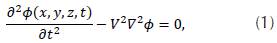
where V is the velocity, which depends on spatial coordinates, and ϕ is the wave function. Considering some boundaries and initial conditions, such as:
where E represents the spatial coordinates, and ∂E is the E boundary; also f(E),g(E) are the known functions in the entire domain. In Cartesian coordinates (x, y, z) and considering integers (i, j, k, n), so that
with the soace and time discretized. Using Taylor series expansion with a fourth order approximation we obtain:
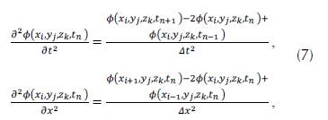
for the coordinates y and z we obtain analogous expressions. By replacing the equation system (7) in (1), solving 𝜙(𝑥i, 𝑦j, 𝑧k, 𝑡n+1) , and following the nomenclature proposed by Yee (1966), we obtain:
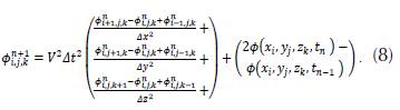
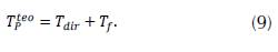
Equation (8) solves the wave equation if the values in the boundary and the initial conditions are known. The elements of the wave function in the time step n + 1 depend on the four nearest neighbors in a previous time step n and on the same component in a time step n - 1. The direct algorithm estimates the arrival time of a seismic wave (T dir ), with propagation from the source j to the station k. The theoretical wave time (P) is obtained aggregating T dir with the time of the seismic event (Tf), as can be seen in (9):
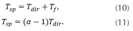
The theoretical calculation of wave time S assumes that the wave velocities S and P are proportional in the entire medium and behave like a Poison solid (10), with proportionality constant with
 . Thus, Ts
teo = αT
dir
- T
f
and the difference of arrival times of waves S and P is:
. Thus, Ts
teo = αT
dir
- T
f
and the difference of arrival times of waves S and P is:
As the station locations are fixed, T dir depends on the velocity distribution and the hypocenter of the seismic event. Therefore T p teo is the only variable that depends on the origin time.
2. Generalized linear inversion
In the inverse algorithm, we compared data measured on the surface with the results obtained from the simulation. Thus, we quantify the difference between the simulated values and the measured observations in the field. Then, it is possible to modify the initial values of the P wave velocity parameters in the field and the coordinates of the hypocenter. With these new initial values, we simulate the arrival times of the P wave for each one of the seismic events and compare the new results with the measured data on the surface, obtaining a new error difference, which will allow us to recalculate the new initial parameters for the next simulation.
This new methodology iterates until the difference between the simulated and the observed data on the surface is lower than the set threshold, in order to invert the velocity, the hypocenter and the origin time simultaneously and the origin time (Crosson, 1976; Ramadan, 2016). In the same way, the hypocenters inversion method was generalized in a simultaneous inversion of velocities and hypo-centers (Franco et al., 2006).
In the model, we consider N seismic sources with hypocenters given by x j = longitude, y j = latitude, z j . = depth, and arrival times t j , where j = {1,2,3...,N}. Additionally, we split the in L blocks space each block with velocity v. , where l = {1,2,3...,L}. These variables compose the model m0:

where 4N + L represents the number of elements.
To determine m 0 , we consider M stations (k = 1,2,...,M) located at (x k ,y k , z k , t k ) and the arrival time observed in the k-th position for the j-th source. A functional relationship T(m 0 ) allows us to reproduce the observed times according to the model m 0 . If this relation is linear, the sensitivity matrix defined as:
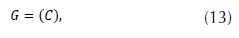
where A j . is a MX4 matrix given by:

and C is a NMxL matrix, the i-th line of C is:
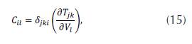
with i(j,k) = k + (j-l)M and δ jki is.
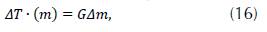
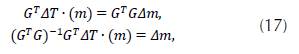
To find Δm (16), we need to invert G, but G is not necessarily a square matrix. Therefore, we use the least square method to determine m, which consists of multiplying the matrix by its transpose and then we invert the result. According to this, (16) is transformed into:
where ΔT is the variation between the time observed (measured on the surface) and the time simulated:
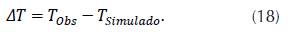
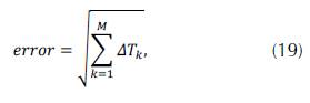
The error between both times is calculated as follows:
and Δm is the change of the model, thus:

The matrix G T G may have determinant equal zero, in which case the matrix is not invertible; this is means that the system shown in (20) does not have a unique solution, and there is at least one null eigenvalue. As proved by Schwerdtfeger (Schwerdtfeger, 1960), there is a method to obtain the subspace solution to the highest likely dimension, known as Lanczos breakdown. This technique consists of decomposing G through matrices built with eigenvalues different from zero. The generalized inverse found with this method fits better the data on the model. However, the computational method cost makes it difficult when implementing real-world applications where matrices are bigger. Furthermore, there is difficulty to formally organize the eigenvalues, due to the data uncertainty because some of them may have values too close to zero to be significant. Therefore, we use a different approach to overcome this obstacle: a weight matrix Є 2 W m is added to the G T G as shown in (21):
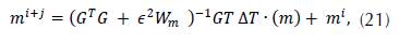
where Є is the dampening factor. If e increases, the error curve presents fewer fluctuations because it depends on the iteration. This factor is found empirically, so we obtained a reasonable fit between the theoretical and observed data, and we also found that the variations of the model during each iteration are small. The W m matrix in the most straightforward cases is the identity matrix. The initial model m 0 is proposed randomly but within a range of values that make sense in the geological model. With this model, the arrival time is simulated with the direct model and is obtained the difference with the reference time ΔT 0 .
It is possible to define the smoothing matrix (Stein & Wysession, s. f.) to modify the change rate of the velocity model. For a 3D geometry composed by a rectangle with several blocks I = L x x l y x L z , the number of columns for D is L and has the following form:
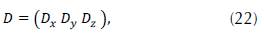
where the sub-matrices D x , D y and D z represent the first derivative in the directions x,y and z with the number of rows (L x -1)L y L z ,L x {l y - 1)L z and L x L y (L z - 1) , respectively. The smoothing is applied to the velocity distribution, so it does not affect the hypocenter and origin time model, hence:
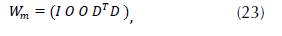
where I is the identity matrix with dimensions 4N x 4N
D x , D y , and D comprise the sub-matrices B x , B y , and B z , defined as:
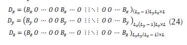
where,
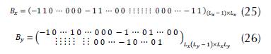
Usually, B x , B y , and Bz, are equal, and the only difference is the separation of the columns between -1 and 1. For B x there is no separation; for B y the separation is L x ; and for B z separation is L x L y .
3. CONDITIONS OF NON-REFLECTIVE BOUNDARY
The boundary conditions known as Dirichlet or Neumann are the most used in the solution of partial differential equations. These boundary conditions can reflect all the energy in the boundary. However, the algorithm determine this energy reflected from any seismic source directly, causing phantom seismic events. Thus, we propose to use non-reflective boundaries, described below.
3.1 Disconnected wave equation
Hastings et. al. (Hastings et al., 1996) proposed a method based on (Berenger, 1994a) that consists of defining potential and decompose the wave equation according to the formulation of (Yee, 1966), is used for the electromagnetic fields.
The wave equation (1) can be split in connected equations, assuming that V is constant. Potential is defined as H = (Hx, Hy, Bz) so that:
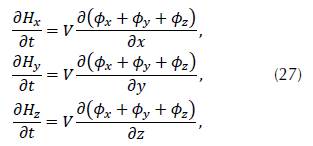
also,
where 𝜙 = 𝜙 x + 𝜙 y + 𝜙 z .
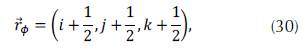
Following the scheme used by (Yee, 1966), the following nomenclature for the indeces is defined as:
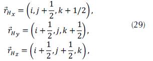
and,
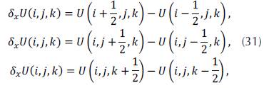
as suggested by Gonzalez (2012), the operators of centered difference are defined as:
According to the equations (30) to (32), the discretization of (27) in Taylor series with second order truncation error is:
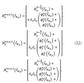
and the discretization for the system shown in (28) is:
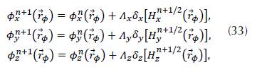
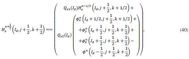
Equations (32) and (33) show the evolution rule, as well as the relation between the potential and the wave function with their neighbors.
Each component of the potential contributed to the full wave function in the corresponding direction (Figure 1 ).
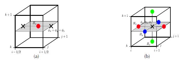
Figure 1: Spatial discretization diagram for the wave equation solution: Circles represent potential, Hx (red), Hy (blue) and Hz (green), and the cross shows the wave function. (a) Relation of Hx with its neighbors (the components of the wave function). (b) Association of 𝜙
x
, 𝜙 y, and 𝜙
z
with its respective neighbors (the potential of each case). When the space split, and the disconnected wave function is in the semi-entire points and around the corresponding potential, which is going to help define its value.
3.2. Attenuation factors
Assuming that the space formed by a square and covered by a shell of determined width, we define an inside region called PML and a contact region called interface (Figure 2). So that one wave will expand freely in the interface and will be absorbed in the PML region.
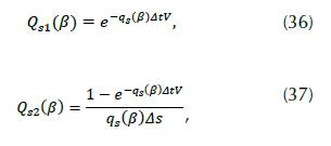
So that the wave attenuation occurs, (Berenger, 1994b) proposes attenuation factors Q s1 and Q s2 in the (33) and (34), so the potential is redefined as:
and for the disconnected wave function:
The attenuation factors
where s = {x,y, z} and β = {i, j, k}, respectively, and
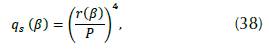
where P is the length of the PML region and r(β) is the depth from the interface to the outside edge as shown in Figure 2(a) and 2(b).
3.3. Complete solution
There is a slight change in the interface between the two regions, and the wave is slowly absorbed depending on the length P. Given the calculated limit in (38), when r → 0 then q → 0. So, from the (36) and (37) it is obtained that Q s1 → 1 and Q s2 → A s thus the same (32) and (33) are reproduced. Then, we use the standard solution in the inside region by using finite differences (8) and redefining the indices following the diagram in (Kane Yee, 1966):
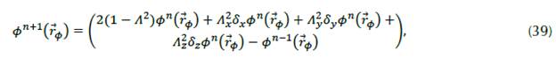
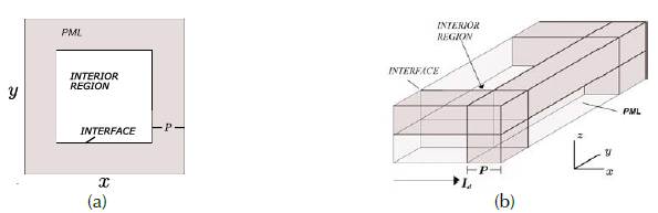
Figure 2: Wave space expansion. (a) The cube is cut in the z axis and forms a plane (known as a slice). A dark color represents the PML region. (b) Upper right edge of the cube.
In the PML region, we use the solution of the disconnected wave equation (35), as well as the following equation in the interface:
where I d is the value that the index i takes in the right-side interface (Figure 2). Similarly, the equation of potential Hx is obtained in the left interface and for the rest of the potentials Hy and Hz. In other words, we have both the potential and the disconnected wave function in the PML region. In the interface we have only the potential and only the wave function in the inside (Figure 3). In most outer boundaries, we can use the Dirichlet or Neumann conditions (2).
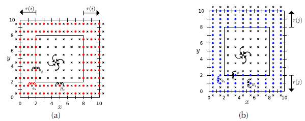
Figure 3: Slices of the cube for the complete solution of the wave expansion with a non-reflective boundary: Circles represent H
x
(red) and H
y
(blue), while crosses represent 𝜙
x
in (a), 𝜙
y
in (b) and 0 (bold cross). Also, the arrows symbolize which neighbor feeds each term and r(β) is the depth of the PML region from the interface to the edge. (a) Discretization for 𝜙x and H
x
. (b) Discretization for 𝜙y and H
y
.
3.4. Scope and limitations
There are three possible limitations in the proposed model. First, the velocity blocks, hypocenters, and stations must be located; then it is possible to define the space and its limits based on those locations. Additionally, the space should be small for a short computational time; conversely, ample space contains the location of elements and stations of the model and allows achieving an equilibrium. Second, it is better to have many blocks for the tomography in order to be more detailed; however, there is a limit to the information available. Finally, since the stations are located on the surface and the hypocenter is distributed in the sub-surface, there is significant uncertainty of the velocity solution the larger the distance between the stations and the hypocenter.
4. SPACE OF THE MODEL
The model validation comprised 54 seismic events, registered in Uraba, Colombia. We developed a model in which the limits are formed by a cubic surface with height h z , width h x in heading West-East, and length h y heading South-North (Figure 4). It represents a part of the surface and sub-surface of this region, where the hypocenters of seismic events, the stations, and the velocity blocks are determined by the user. Furthermore, h x and h y are given by the location of the stations and epicenters of the seismic events (superficial projection of the hypocenters), while h z is limited by the distribution of these events.
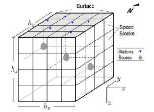
Figure 4: Spatial limits of the model formed by one cube split into blocks L with N sources and M stations.
4.1. Number of elements in the model
There is a limit for the number of elements considered in the model depending on the information available. According to the number of seismic events (N = 54), 403 observed times are determined (number of equations), including the arrival time of the P wave (TP) and the difference between the arrival times of the P and S waves (TSP). To have a better adjustment of the convergence of the generalized inversion corresponding to the observed information, the number of equations cannot exceed the number of unknown factors; otherwise, we obtain unexpected solutions. The unknown factors are the elements of the model; for every seismic event there are 4 (location x; y; z of the hypocenter and origin time), that is 4 x N = 216. They reduce the number of blocks to consider:
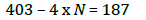
So, the maximum number of blocks is 187. If hx, h y , and h z split up in Lx, Ly, and L z intervals, then a matrix forms a L = L x xL y x L z total blocks, so that L x xL y x L < 187.
4.2. Uncertainty of the velocity with depth
The last limitation is the uncertainty of velocity with depth. The trajectory between the hypocenter and the station is named ray according to the Fermat principle: the way taken by a wave expanding from one point to the other is such that the time used to cover it is minimum. The more significant the depth, the littler the ray density; so, the deepest cubes have a lower possibility of being crossed by a ray; furtherore, the uncertainty of velocity is more significant.
5. DIRECT ALGORITHM VALIDATION AND THE NON-REFLECTIVE BOUNDARIES
A region built with dimensions 200km x 40 km x 40km and seven stations on the surface, 10km apart towards x starting from x = 20km and the seismic source at (100, 25, 25) km, with velocity V p = 5km/s as shown in Figure 5(a).
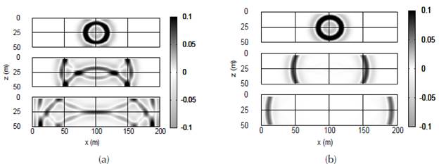
Figure 5: Plane viewy = 25 km.
(a) Without boundaries PML. (b) With boundaries PML.
Figure 5(a) shows the wave reflecting on the boundary, while in figure 5(b) the wavefield is like an open frontier. These reflections to the inside of the region in the study do not appear.
6. VALIDATION OF THE INVERSION PROGRAM
We built a synthetic model considering a region with dimensions 48km x 48 km x 48km divided into 64 blocks, each one characterized by velocity. The distribution is analogous to the checkerboard, with the alternate velocity 5.5 km/sand 6.5 km/s. In each block, a seismic source is at the center, and 16 stations in the center of the upper face of the superficial blocks as shown in Figure 6(a).
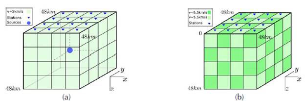
Figure 6: (a) Reference synthetic model containing 64 blocks with alternate velocity 5.5km/s and 6.5 km/s, 16 stations in the surface (blue triangles), and 64 seisms in the center of each block. (b) Model with homogeneous velocity of (5km/s) and initial location of the sources in the center of the cube.
Using the direct algorithm, we simulate seismic events and determine the arrival times for each one (T obs).
We run the initial inverse algorithm assuming an initial model with a uniform velocity of 5 km/s and hypocenters located in the center of the region (24 x 24 x24) km (Figure 6(b)). As expected, the initial error is significant. Figure 7(a) shows the result of 69 iterations where the error given by (21) converges after a certain number of iterations and the model does not change significantly. It was comparing the synthetic model in Figure 6(a) with the final model in Figure 7(b), it is possible to see that the difference is minimal on the surface but increases in deep parts and even more in the corners (Figure 8). Similarly, the error related to the velocity distribution increases the deeper the hypocenter is located (Figure 7). This distribution means that a deep block has less chance to be sampled by the wave of any sources, and it will weigh less in the solution of the inversion. Therefore, a deep source location error because of the velocity error of a deep block.

Figure 7: (a) Error variations depending on the iterations for a model with constant velocity. (b) Final model after the inversion containing 64 blocks, 16 stations in the surface, and 64 hypocenters (one per each block). (c) Slice of the hypocenters projections on the xy surface (z = 0). (d) View of the hypocenters projections in the xz plane (y = 0).
Figure 7(c) shows the the hypocenters in the plane xy (Slice z = 0). They are located approximately in the center of the block, like the reference model. In Figure 7(d), we have the projections of the locations over the plane xz (y = 0), where the hypocenters are approximately in the center of each block, except for the deepest blocks. The black dots show a more significant error.
A lack of information produces errors in the locations as well as errors in the estimation of velocity. This error is due to the ray paths coming to form seismic events that cut the blocks in the surface, while deeper rays only cuts deepest blocks. This lack of information from the deepest blocks creates an error in the source location of the sources, as well as higher velocities (Figure 8). In Figures 8(a) to 8(c), the slices of the more superficial layers show that the velocity value is close to the value calculated by the reference model (Figure 6(a)), but Figure 8(d) represents a deeper layer, and the values show a more significant error.
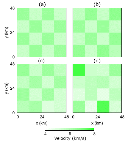
Figure 8: Velocity Slice section to different depths (a)
CONCLUSIONS
An inversion program was created using inverse and direct models of an algorithm with the following contributions: the inverse algorithm considers the smooth velocity variations found in the geological models, while the direct algorithm works with finite differences and non-reflective PML boundaries, which offers a useful tool to make high-quality synthetic seismograms.
In order to prove the direct algorithm, we suggest making the solution of the wave equation by finite differences with non-reflective boundaries and truncation error of grade 4 or higher. This reduces the error of the theoretical arrival time without damaging the computational time.
Multiple sources run simultaneously; this would represent a significant advance. For this reason, we proposed that the sources be distinguished by their frequency, as is the case with FM radio stations. Then, the simulated stations must discriminate frequencies, so that the computational time decreases.
Better results may be achieved if the acquisition time had been more significant. Therefore, we propose to install stations in the zone for over a minimum of 5 years. We also recommended the inversion program in real-time, with this work as an initial model, and obtaining a better resolution of the velocity and a reinforce the understanding of the tectonics of the region. The inversion program can be used for stations without synchrony.
REFERENCES
License
Esta licencia permite a otros remezclar, adaptar y desarrollar su trabajo incluso con fines comerciales, siempre que le den crédito y concedan licencias para sus nuevas creaciones bajo los mismos términos. Esta licencia a menudo se compara con las licencias de software libre y de código abierto “copyleft”. Todos los trabajos nuevos basados en el tuyo tendrán la misma licencia, por lo que cualquier derivado también permitirá el uso comercial. Esta es la licencia utilizada por Wikipedia y se recomienda para materiales que se beneficiarían al incorporar contenido de Wikipedia y proyectos con licencias similares.