DOI:
https://doi.org/10.14483/23448393.18466Publicado:
2022-01-04Número:
Vol. 27 Núm. 1 (2022): Enero-AbrilSección:
Sección Especial: Mejores artículos extendidos - WEA 2021Evaluation of the Accuracy of the Sound Field Separation Method under Variations in the Location of the Sampling Points
Evaluación de la precisión del método de separación de campos sonoros bajo variaciones en la ubicación de los puntos de muestreo
Palabras clave:
sound field separation, acoustic radiation, spherical harmonics (en).Palabras clave:
separación de campos sonoros, radiación acústica, armónicos esféricos (es).Descargas
Referencias
R. Heyser, “Acoustical Measurements by Time Delay Spectrometry,” J. Audio Eng. Soc. vol. 15, no. 4, pp. 370-382, 1967.
J. M. Berman and L. R. Fincham, “Application of Digital Techniques to the Measurement of Loudspeakers,” J. Audio Eng. Soc., vol. 25, no. 6, pp. 370-384, 1977.
E. G. Williams, J. D. Maynard, and E. Skudrzyk, “Sound source reconstructions using a microphone array,” J. Acoust. Soc. Am., vol. 68, no. 1, pp. 340-344, 1980. https://doi.org/10.1121/1.384602 DOI: https://doi.org/10.1121/1.384602
D. Keele Jr., B. Don, H. Lu, and S. Wu, “High-accuracy full-sphere electro acoustic polar measurements at high frequencies using the HELS method,” in Audio Engineering Society Convention 121, San Francisco, CA, USA, 2006.
G. Weinreich and E. B. Arnold, “Method for measuring acoustic radiation fields,” J. Acoust. Soc. Am., vol. 68, no. 2, pp. 404-411, 1980. https://doi.org/10.1121/1.384751 DOI: https://doi.org/10.1121/1.384751
E. G. Williams, Fourier Acoustics: Sound Radiation and Near-field Acoustic Holography, Cambridge, MA, USA: Academic Press, 1999.
M. Melon, C. Langrenne, D. Rousseau, and P. Herzog, “Comparison of four subwoofer measurement techniques,” J. Audio Eng. Soc., vol. 55 no. 12, pp. 1077-1091, 2007.
W. B. Li, M. Z. Lian, C. X. Bi, J. Chen, and X. Z. Chen, “Separation theory of the incident and scattered sound fields in spherical coordinate,” Sci. China, Ser. E Technol. Sci., vol. 50, no. 3, pp. 631-370, 2007. https://doi.org/10.1007/s11431-007-0014-4 DOI: https://doi.org/10.1007/s11431-007-0014-4
A. Fahim, P. N. Samarasinghe, and T. D. Abhayapala, “PSD Estimation and Source Separation in a Noisy Reverberant Environment Using a Spherical Microphone Array,” in IEEE/ACM Transactions on audio, speech, and language processing, 2018. DOI: https://doi.org/10.1109/WASPAA.2017.8169998
A. Amir, J. Ahrens, M. Geier, S. Spors, H. Wierstorf, and B. Rafaely, “Spatial perception of sound fields recorded by spherical microphone arrays with varying spatial resolution,” J. Acoust. Soc. Am., vol. 133, no. 5, May 2013. https://doi.org/10.1121/1.4795780 DOI: https://doi.org/10.1121/1.4795780
P. Zhang, Z. Kuang, M. Wu, and J. Yang, “A novel method for measuring acoustic radiation fields of subwoofers based on non free-field aspheric measurements,” International Congress on Sound and Vibration, 2014.
P. Zhang and X. Bi, “Patch nearfield acoustic holography combined with sound field separation technique applied to non-free field,” Sci. China Phys. Mech. Astr., vol. 58, no. 2, pp. 1-9, Aug. 2014. https://doi.org/10.1007/s11433-014-5467-4 DOI: https://doi.org/10.1007/s11433-014-5467-4
Cómo citar
APA
ACM
ACS
ABNT
Chicago
Harvard
IEEE
MLA
Turabian
Vancouver
Descargar cita
Recibido: 15 de agosto de 2021; Aceptado: 15 de septiembre de 2021
Abstract
Context:
Measuring the directivity characteristics and the frequency response of acoustic sources is a difficult process, as the dimensions and boundary conditions of the testing rooms used could constrain the measurement procedure. The testing room should guarantee a free-field condition, which is usually satisfied by using big acoustic absorbers with fibrous materials with high absorption coefficients. Ho wever, standing wave patterns can be easily developed due to the frequency range exciting the testing room.
Method:
The sound field separation method can isolate the radiated field of an acoustic source by sampling the sound field around it over two holographic spheres. The coordinates of the sampling points are used in a set of equations, whose solution can estimate the radiated field. In this paper, the effect of the variability on the actual positions of these sampling points is investigated.
Results:
Two numerical simulations with and without external sources outside the holographic spheres were performed. In all simulations, variations in the radial position of the sampling points were induced, and the relative reconstruction error, the directivity index, and the frequency response were studied. The results indicate that, for estimating the directivity of low-frequency acoustic sources, regardless of the presence of external sources, radial positioning of the sensors does not have to be exact to obtain an accurate reconstruction.
Conclusions:
This study suggests that, in the experimental characterization in conventional testing rooms of the radiated field from acoustic sources whose main frequency region corresponds to low frequencies, e.g. subwoofers, the SFS method could be used, thus obtaining high accuracy in the estimation of the directivity of the source.
Keywords:
sound field separation, acoustic radiation, spherical harmonics..Resumen
Contexto:
La medición de las características de directividad y de respuesta en frecuencia de fuentes acústicas es un procedimiento difícil debido a que las dimensiones y condiciones de frontera del recinto dentro del cual se hace el ensayo podrían limitar el procedimiento de medición. El recinto de ensayo debería garantizar condición de campo libre, lo cual se consigue usualmente con absortores acústicos de gran dimensión hechos de materiales fibrosos con altos coeficientes de absorción. Sin embargo, se pueden desarrollar con facilidad patrones de ondas estacionarias debido al rango de frecuencia que hace vibrar el recinto de ensayo.
Método:
El método de separación de campos sonoros puede aislar el campo irradiado por una fuente acústica a través del muestreo del campo sonoro alrededor de ella en dos esferas holográficas. Las coordenadas de los puntos de muestreo se usan en un conjunto de ecuaciones cuya solución permite estimar el campo irradiado. En este artículo se investiga el efecto de la variación en las posiciones reales de los puntos de muestreo.
Resultados:
Se hicieron dos simulaciones numéricas fuera de las esferas holográficas, una sin fuentes externas y otra con fuentes externas. En todas las simulaciones se indujeron variaciones en las posiciones radiales de los puntos de muestreo y se estimaron el error relativo de reconstrucción, el índice de directividad y la respuesta de frecuencia. Los resultados indican que, para estimar el índice de directividad de fuentes acústicas de bajas frecuencias, independientemente de la presencia de fuentes externas, la posición radial de los sensores no tiene que ser exacta para lograr una estimación precisa.
Conclusiones:
Este estudio sugiere que, en la caracterización experimental en recintos convencionales del campo irradiado por fuentes acústicas cuyo rango de frecuencia predominante es el de bajas frecuencias, por ejemplo, subwoofers, el método de separación de campos puede ser usado, obteniendo resultados de alta precisión en la estimación de la directividad de la fuente.
Palabras clave:
separación de campos sonoros, radiación acústica, armónicos esféricos..Introduction
The experimental characterization of sound fields from acoustic sources radiating in the low frequency range, such as the case of subwoofer speakers, poses a physical limitation since the dimensions of the testing rooms that guarantee free-field conditions, i.e., anechoic chambers, must be larger than a quarter of the wavelength λ of the lowest frequency of interest and there are no testing rooms big enough to satisfy this condition. Additionally, due to the frequency range of the sound field radiated by a subwoofer speaker, standing waves can easily be generated in such rooms, thus infringing the free-field condition by the superposition of the standing waves with the radiated field. The fibrous materials present in the testing room to control reverberation and guarantee freefield conditions should have dimensions comparable to the wavelength of the lowest frequency of interest, thus forcing these elements to be robust and big while making the realization of free-field conditions difficult.
Several methods have been proposed in the past to overcome the difficulties stated above. Some of them try to isolate the reflections from the testing room by applying a time window to the impulse response estimated when the acoustic source is radiating in the room 1, 2. However, special care should be taken while selecting a testing room big enough, so that the early reflections do not overlap with the direct energy from the source.
The development of the Near-field Acoustic Holography (NAH) technique 3 allowed the possibility to decompose a radiated sound field from a source in terms of plane waves by sampling the acoustic pressure in the near field. By separating the forward and backward propagating fields, the radiated field can be estimated. Other methods such as the Helmholtz equation least-square (HELS) in 4 showed significant accuracy while estimating the directivity of the pressure field radiated by a rectangular plate.
In 1980, 5 formulated and experimentally applied the Sound Field Separation (SFS) method, where, by means of an expansion of the sound field in terms of spherical waves as described in 6, the outward and inward propagating fields can be estimated. With this separation of fields, the radiated field of an acoustic source was estimated in the near field, thus avoiding the guarantee of having free-field conditions and allowing the estimation of the acoustic radiation in normal rooms. 7) compared four different techniques to measure the frequency response and directivity of subwoofer speakers. The evaluated methods were the measurement of a subwoofer in an anechoic chamber, in a pseudo-free field, in a reference chamber, and with the SFS method. By comparing the data obtained from the experimental characterization with each method, the SFS method proved to be the most accurate at estimating the radiated field. Other application areas of the SFS method include the estimation of the scattered sound field from a rigid sphere under the incident propagation of a spherical sound field 8. In recent years, several methods have been proposed to estimate characteristics of an acoustic signal using a decomposition on spherical harmonics, such as the estimation of the power spectral density (9) and spatial perception of a source (10. In their research, (10 propose a novel method to measure subwoofers in virtual free-field conditions. Such conditions are achieved precisely by separating the sound fields of several sources into spherical harmonics and then reconstructing the field of the single source in question, which was placed inside a spherical sensor array in 11. According to the above, field separation allows characterizing acoustic sources in spaces where it is usually not possible due to disturbances in the sound field. Finally, (12 propose an experiment in which they combine near-field acoustic holography with a field separation method, so that it can be determined how convenient it is to use the NAH method with a double layer of sensors in environments characterized by not being in free field. It is concluded that the method works by largely eliminating interference from other sources and reconstructing the field of the source in question. At the same time, they determine that, when performing this experiment with a single layer of sensors, it is not possible to determine the position of the source under analysis, especially at high frequencies; while, using a double layer of sensors, it is possible to reconstruct the sound field 12.
The basic principle in the application of the SFS method is the use of a dual-layer measurement sphere, from now on called ‘holographic spheres’. By sampling the acoustic field over these holographic spheres and decomposing the total field in terms of spherical waves, the incoming and outgoing propagating fields can be estimated. However, the exact location of each sampling point (measurement point) must be accurately known in order to reconstruct the outgoing field, as the analytical expansion method estimates the radial magnitude and phase shift in each measured direction. This study aims at evaluating, by means of numerical simulations, the accuracy of the SFS method in the reconstruction of the radiated field from an acoustic source with the presence of variation in the radial location of the sampling points. This, to simulate a real-life application where the sampling points are not placed accurately.
This research paper is organized as follows: the theoretical background (Section 2) of the expansion of a sound field in terms of spherical waves and the mathematical procedure of the SFS method is described in section. The configuration, problem statements, and indexes for evaluation for the numerical simulations are addressed in Section 3. Section 4 presents the results and discussion of the numerical simulations. Finally, in Section 5, the conclusions of the study are presented.
Theoretical background
Sound field representation in spherical coordinates
The acoustic pressure p(k, r, θ, φ) of a sound field propagating in a medium can be represented in spherical coordinates as

and h (2) n is the spherical Hankel function of the second kind and order n, which represents the incoming spherical waves. Cmn and Dmn are coefficients weighting each term of the spherical wave expansion. k = ω/c is the wavenumber corresponding to the ratio of the angular frequency ω with respect to the propagating speed of sound c. Y m n are the spherical harmonics, defined as

with i being the imaginary unit, and P m n (cos θ) the associated Legendre function. The spherical wave spectrum Pmn(k, r) of the sound field p(k, r, θφ) at a distance r can be defined as

where (·) ∗ denotes the complex conjugate operator. Eq. (3) can be regarded as the forward Fourier transform with basis function Y m n (θ, φ), and the corresponding inverse Fourier transform is

Fig. 1 shows an acoustic source Π of arbitrary shape radiating a sound field. The radiated sound field can be expressed according to Eq. (1) at two holographic (measurement) spheres of radii r1 and r2, thus obtaining p(k, r1, θ, φ) and p(k, r2, θ, φ), respectively. The spherical wave spectrum Pmn(k, r) of the acoustic pressures of each of these holographic spheres can be estimated by means of Eq. (3), thus obtaining Pmn(k, r1) and Pmn(k, r2). These spherical wave spectrums are related to each other by the extrapolation principle of the wavefield as


Figure 1: Holographic measurement planes located at radii r1 and r2 8
with hn(kr) being the spherical Hankel function of the first or second kind.
Sound field separation theory
The main objective in the application of the sound field separation (SFS) technique corresponds to the reconstruction of the outgoing wavefield radiated by an acoustic source propagating in a domain with non-free-field boundary conditions. The acoustic pressure p(k, r, θ, φ) at a holographic sphere with radius r around the acoustic source Π can be represented according to Eqs. (1) and (4), as

thus, representing the superposition of outgoing and incoming spherical waves in the spherical wave spectrum Pmn(k, r).
As the radiated sound field from the acoustic source only contains outgoing spherical waves, the spherical wave spectrum of the radiated field P O mn(k, r) can be defined as

When two holographic spheres with radii r1 and r2 are used, as shown in Fig. 1, the spherical wave spectrums of the radiated field are related following Eqs. (5) and (7), as

The reflected acoustic field contains outgoing and incoming spherical waves, which can be represented with the spherical wave spectrum

expressed according to Eq. (6). The spherical Hankel function of the first and second kind, h (1) n and hn, respectively, can be expressed as

with jn and yn being the spherical Bessel functions of the first and second kind, respectively. The substitution of Eq. (10) into (9) yields

The functional behavior of the spherical Bessel function of the second kind yn indicates that, when the radius of the holographic sphere r = 0, yn(0) → −∞. However, as the acoustic field at such position must be finite, then AI mn = C I mn to satisfy this physical condition.
The spherical wave spectrum of the total acoustic field Pmn at the holographic spheres in Fig. 1 becomes


by combining Eqs. (7), (8), and (9). The coefficients for the outgoing waves of the total acoustic field are AT mn = AO mn + AI mn. Recalling that AI mn = C I mn in order to guarantee a finite sound field at r = 0, then AOmn = AT mn − C I mn. Solving for AT mn and Cmn from Eqs. (12) and (13) yields


Recalling Eq. (8), if the radiated sound field from the acoustic source were to be estimated at a reconstruction sphere with radius r = r0, the spherical wave spectrum would be

Finally, the acoustic pressure radiated from the source can be estimated using the inverse Fourier transform in Eq. (4) using the spherical wave spectrum from the radiated field P O mn(k, r0) from Eq. (16).
Singularity of the sound field separation method
A key aspect in the estimation of the acoustic pressure radiated from the source is the calculation of the weighting coefficients AT mn and C I mn according to Eqs. (14) and (15), respectively, where both equations have the same denominator. The behavior of the denominator will constrain the stability of the estimation of the radiated field, as there might be values for kr where both Eqs. (14) and (15) might become singular 8.
Recalling Eq. (10), the following relationship between the spherical Hankel functions of the first and second kind can be established:

Therefore, the denominator in Eqs. (14) and (15) can be expressed in terms of (17), thus yielding
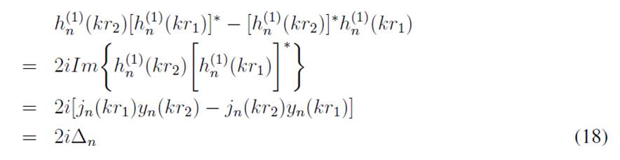
Therefore, Eq. (18) will exhibit a singular behavior under certain values for the variables k, r1 and r2, which are dependent on the separation distance between the holographic spheres d = r2 − r1. Fig. 2 shows the functional behavior of ∆n in Eq. (18), where the zero-crossing points have been marked. It can be observed that, for a separation distance (d = 0, 1 m), the first zero-crossing point occurs at 1.716,6 Hz, whereas, for (d = 0, 2 m), it is located at 860,4 Hz. Then, the first singular point can be shifted to higher frequencies by decreasing the separation distance between the holographic spheres d, thus implying that, when d λ, where λ is the wavelength of the highest frequency of interest, the frequency range of the reconstruction can be extended.
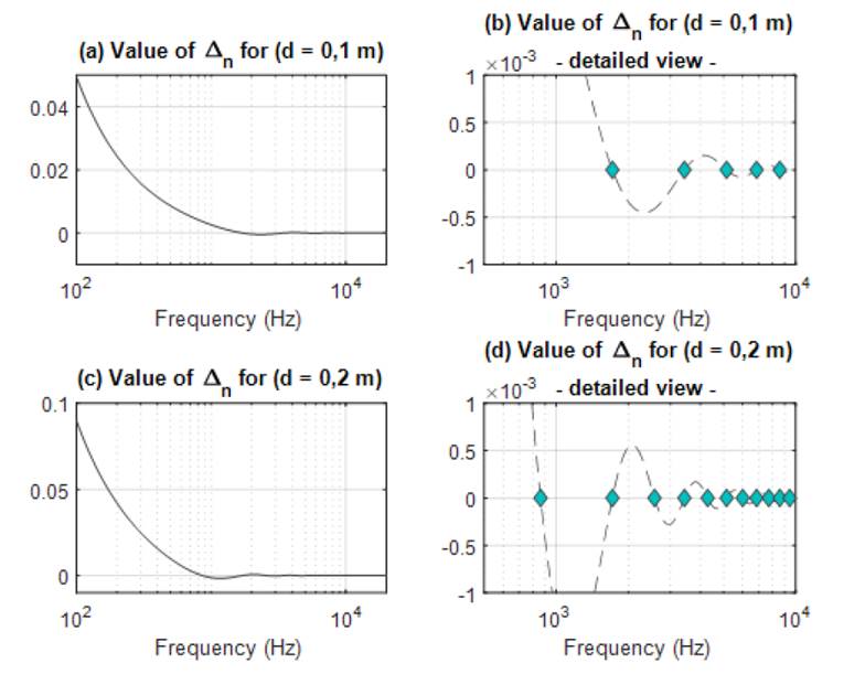
Figure 2: Singular behavior of the denominator in Eqs. (14) and (15) for a separation distance between the holographic spheres as (d = 0, 1 cm) (top) and (d = 0, 2 m) (bottom). Zero-crossing points marked with () in (b) and (d).
Sound field separation with finite sampling points
The representation of the acoustic pressure radiated by the source according to the inverse Fourier transform in Eq. (4) indicates that it is necessary to consider an infinite number of terms in order to properly represent the acoustic field p(k, r, θ, φ) in terms of the spherical wave spectrum Pmn(k, r) and the spherical harmonics Y m n (θ, φ). On the other hand, Eq. (3) can be regarded as the representation of the acoustic pressure over a continuous holographic sphere.
In practice, the two holographic spheres with radii r1 and r2 would be discretized with M sampling points, so that each point over the sphere would be located at (ηl , θl , φl) with l = 1, 2, . . . , M. The order η of the expansion in Eq. (4) would be truncated to an order N, so it would be expressed as

representing a finite set of linear equations, of which Pmn(k, rl) are unknowns that should be determined. A least-squares solution for this set of linear equations can be applied to solve for the spherical wave spectrums Pmn(k, rl). However, in order to guarantee the existence of a least squares solution, the system must be overdetermined, thus implying that the number of sampling points M must be equal to or greater than the number of unknows. Recalling that, for each spherical wave spectrum Pmn(k, r), a pair of Amn and Cmn coefficients could be needed. The total amount of unknows to be determined equals 2(N + 1)2 , so that the least-squares solution can be estimated if M ≥ 2(N + 1)2 . Eq. (19) can be written in matrix form:

from which the least-squares solution for the vector pmn is given by

Numerical simulation
This section describes the configuration given to different parameters involved in the SFS method. The objective of the study was to evaluate the accuracy of the reconstruction of the radiated field by an acoustic source, located at the center of two holographic spheres, under the presence of variations in the location of the sampling points around said spheres, while assuming that the actual location of each sampling point was the same as the one used in the reconstruction of the field. The intention was to simulate a real-life application, where the distances rl of each sampling point used in the reconstruction procedure described in Section 2.2 are different to the real positions used during the measurement. To this effect, two numerical simulations were performed in MATLAB. The first simulation consisted of the reconstruction of a radiated field under free-field conditions without the presence of any other source. The second simulation aimed at reconstructing the same radiated field while other acoustic sources were located outside the farthest holographic sphere. This, to simulate the presence of external sources that would contaminate the sampled acoustic field by propagating incoming spherical waves into the holographic spheres. For each simulation, the same amounts of variation on the distances rl of the measurement points were induced. The problem statements and configurations for each numerical simulation are presented in Section 3.1, and the indexes for the evaluation in Section 3.2.
Stating the problema
Simulation without external sources
The first simulation consisted of the reconstruction of the sound field radiated by an acoustic source located at the center of two holographic spheres. A monopole source was located at the origin of the coordinate system. The acoustic radiation from the monopole source was set in such a way that a sound pressure level of 94 dB would be obtained 1 m away from the source for all the frequencies under free-field conditions, i.e., the spectrum from the radiated field would be flat in all frequencies. As the radiated field is symmetrical in all directions, the estimation can be studied only in the horizontal orbit by setting the elevation of all the sampling as θl = 0. A first set of sampling points was distributed over a holographic sphere, whose center was located at the same position of the monopole source. The radius of this sphere was set to r1 = 1 m, so the distances of all the sampling points over this sphere would be at 1 m. A second set of sampling points was located at a second holographic sphere with a radius r2 = 1, 2 m, so the two holographic spheres were separated with a distance d = r2 − r1 = 0, 2 m.
The angular separation between the sampling points over each holographic sphere was determined to replicate a conventional measurement procedure, where an angular resolution of ∆θ = 5◦ is commonly used. In this way, there were 71 sampling points, so the order of the spherical wave expansion in Eq. (19) would be N = 5.
Simulation with external sources
The configuration in terms of the location of the radiating source and the sampling points for the second simulation was the same as the one described in the previous section. In this case, the only difference corresponded to the addition of eight monopole sources located as shown in Fig. 3. The location of these additional monopole sources was set outside the holographic sphere, whose radius was r2 = 1, 2 m.
The goal with this distribution of the sources was to simulate the presence of external sources that would contaminate the radiated acoustic field to later evaluate the performance of the SFS method. The radiation from each of the eight external sources was set in such a way that a sound pressure level of 88 dB would be measured 1 m away from each source. To avoid having correlated external sources, random noise with a standard deviation of 1,0 dB was added to the acoustic pressure of each external source.

Figure 3: Distribution of internal and external sources and sampling points in the second numerical simulation
Variation of the sampling points’ location
To simulate a real-life application where there could be variability in the location of the sampling points during the measurement procedure with respect to the assumed locations used during the SFS method, a random variation in the distances of each sampling point rl was induced. For each of the above-mentioned simulation, the distances rl of each set of sampling points were varied with a normal distribution, whose mean corresponds to the radius of each holographic sphere. Four different standard deviation values were considered: (σr = 0, 0 m, 0, 005 m, 0, 02 m, 0, 05 m).
Indices for evaluation
The evaluation of the performance of the SFS method under the influence of the position variability of the sampling points was conducted by estimating the relative error and comparing the normalized frequency response and directivity index for each standard deviation on both simulations.
Relative error
The error norm used for the evaluation of the performance of the SFS method is the total mean square difference between the theoretical radiated field at each sampling point pl(k, rl , θl , φl) and the reconstructed values p˜l(k, rl , θl , φl), defined as

Normalized frequency response
The frequency response function of the reconstructed field at the axial direction p˜l(k, r1, 0, 0) was normalized with respect to the acoustic pressure radiated by the inner source at 1 kHz, p1kHz(r1, 0, 0) as follows:

Directivity index
Due to the importance of accurately reconstructing the directive characteristics of the radiated field, the directivity index was defined as

where p(k, r1, 0, 0) represents the acoustic pressure of the sampled field in the axial direction, and p(k, r1, θl , φl) is the acoustic pressure at every other position l.
Results and discusión
This section shows the results obtained for the two configurations of the proposed numerical simulations in Section 3. After performing the simulations, several analyses were carried out to understand the different variations in the accuracy of the SFS method. The results for the four standard deviations were overlapped, so that the variations in their behavior could be easily analyzed. First, the relative errors of the reconstruction of the radiated fields for each configuration and standard deviation σr are presented in Section 4.1. Next, the accuracy in the reconstruction of the directive characteristics of the radiated field are addressed in Section 4.2 by estimating the directivity indexes. Finally, Section 4.3 presents the evaluation of the normalized frequency responses reconstructed in the axial direction for each simulation.
Evaluation of the relative error
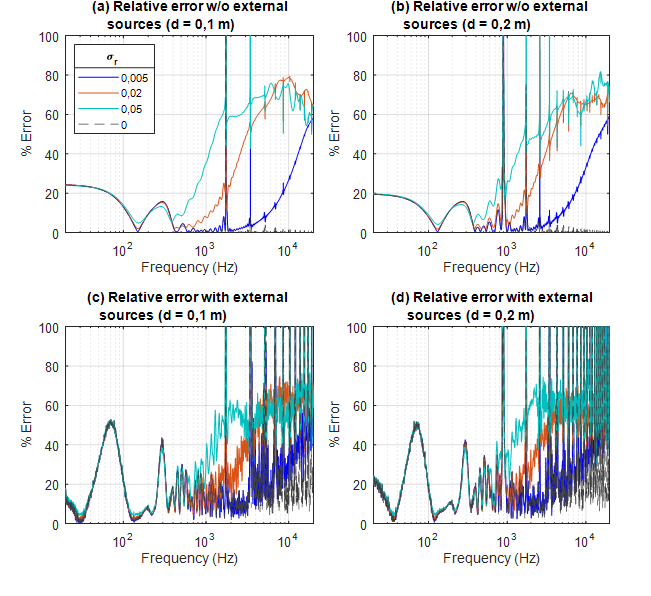
Fig. 4 shows the estimation of the relative error according to Eq. (22). Figs. 4a and b correspond to the estimated error when the radiated sound field is reconstructed without the presence of any external source, as described in Section 3.1. Figs. 4c and d correspond to the estimation of the relative error in the construction of the radiated field under the presence of external sources. The left figures represent the reconstruction with a separation d = 0, 1 m, and right figures d = 0, 2 m. For all possible configurations, the relative error of the reconstruction exhibits a discontinuous behavior beyond certain frequency. For the case where the separation distance corresponds to d = 0, 1 m, this behavior occurs from approximately 1,7 kHz, whereas, for the separation distance of d = 0, 2 m, this cutoff frequency is shifted to a lower range of approximately 860 Hz, which is consistent with the singular behavior described in Section 2.3.
For larger standard deviations, the amount of relative error generally increases at higher frequencies. However, at low frequencies, there is no significant difference between the theoretic and the standard deviations in the different configurations. In Fig. 4b, an acceptable relative error rate of up to 860 Hz with a maximum of 20 % can be seen. In addition, a minimum relative error can be noticed around 130 Hz. Also, a singular behavior starting at 860 Hz is evidenced, where the amplitude tends to increase, and a discontinuous behavior begins.
In Figs. 4c and d, when the external sources are contributing to the pressure field, a ripple appears, and the relative error is significantly increased at low frequencies such as 71,6 Hz and 300 Hz. The trend of standard deviations remains the same, meaning that, while the standard deviation increases, the amount of relative error also increases at higher frequencies. It can also be noticed in Fig. 4d that there is an increase in the relative error of the region above the singular points that first appeared in Fig. 4b, which can be attributed to presence of the external sources influencing the reconstruction accuracy of the SFS method. Additionally, the instability of the approximated solution is determined by the singular behavior described in Section 2.3, which can also be worsened by the least-squares method, recalling that the reconstruction procedure needs to estimate the pseudo-inverse of the matrix Y, as described in Section 2.4. The first peak appears at 71,6 Hz with a relative error of 51 %, more than twice the error observed at the same frequency in the simulation without any external sources. Finally, in Figs. 4a and c, the cutoff frequency from which the singular behavior appears is shifted to a higher frequency with respect to 4b and d, as anticipated in Section 2.3. However, these changes do not seem to affect the trend of the relative error in each standard deviation. The amplitudes of the relative error increased slightly for low frequencies, while they decreased at mid-high frequencies.

Figure 4: Relative error for the different configurations of the numerical simulations. Reconstruction without external sources in (a) and (b), and with external sources radiating in (c) and (d). Separation distance d between the holographic spheres: d = 0, 1 m in (a) and (c), and d = 0, 2 m in (b) and (d).
Evaluation of directivity indexes
In Figs. 5a and b, the directivity index shows consistent values on lower frequencies for each standard deviation, which means that, regardless of the deviations induced in the radial location of the sampling points, the directivity of the source can be properly reconstructed up to a certain frequency. Again, for a separation distance d = 0, 2 m the directivity index presents large variations starting at 900 Hz, whereas decreasing this distance by half (d = 0, 1 m) shows a shift in these variations, which agrees with the relative error described in Section 4.1. It should be noted that the variations are larger, as the standard deviation is also larger. With the presence of external sources, in Figs. 5c and d, the directivity index has the same ripple seen in Fig. 4. For the separation distance d = 0, 2 m, between 200 Hz and 300 Hz, the directivity index starts to deviate from the theoretical value of 0 dB, and, beyond these frequencies, the SFS method fails at reconstructing the directivity of the radiated field. It is important to note that, regardless the value of the standard deviation, the result is the same up to 860 Hz, which suggests that these amounts of standard deviations do not affect accuracy while reconstructing the directivity index.

Figure 5: Estimation of the directivity index for the different configurations of the numerical simulations. Reconstruction without external sources in (a) and (b), and with external sources radiating in (c) and (d). Separation distance d between the holographic spheres: d = 0, 1 m in (a) and (c), and d = 0, 2 m in (b) and (d). The location of the external sources is shown in Fig. 3.
Evaluation of the normalized frequency responses
Finally, Fig. 6 shows the normalized frequency response of the reconstructed field for the different configurations. Here, the frequencies where the singular behavior appears match those in Fig. 4. As expected, when d = 0, 2 m, the first peak appears at 860 Hz, and, for d = 0, 1 m, the peak is shifted to a higher frequency. At low frequencies, the frequency response is almost the same for each standard deviation matching the behavior described in Section 4.1, Fig. 4.
In Fig. 6c, where d = 0, 1 m, there is a slight difference between the magnitude of the frequency responses for each standard deviation in the low frequencies. This is to say, lower distances between the holographic spheres could mean an increase in the contribution of the standard deviations to the normalized frequency response, as these standard deviations σr become comparable with the separation distance between the holographic spheres, d. This suggests that the separation distance between the holographic spheres should be selected with care if the intention is to reconstruct the radiated field in the low frequency region.
As this study is focused on low frequencies, it is necessary to evaluate some critical points. Fig. 4b shows that, at 71,6 Hz, there is a relative error of 14,3 %, which is increased when the external sources contribute to the pressure field, as can be seen in Fig. 4d. However, this amount of error
may be due to variations in the directivity index or the frequency response. Fig. 6d shows that the relative error is due to the frequency response reconstruction. In addition, the frequency with the lower error before the singular behavior appears corresponds to 135,2 Hz. Figs. 5 and 6 validate that the frequency response and the directivity index are properly calculated at 135,2 Hz, regardless of the distance between the holographic spheres or the presence of any external sources. Fig. 6 shows the low accuracy of the SFS method in reconstructing the frequency response, especially at 71,6 Hz. As stated above, this is an important point to analyze, so Fig. 7 shows the polar pattern for this frequency.

Figure 6: Normalized frequency response estimated in the axial direction for the different configurations of the numerical simulations. Reconstruction without external sources in (a) and (b), and with external sources radiating in (c) and (d). For separation distance d between the holographic spheres of d = 0,1 m in (a) and (c), and d = 0,2 m in (b) and (d). The location of the external sources is shown in Fig. 3.
The SFS method at 71,6 Hz appears to properly reconstruct the omnidirectional behavior of the source, albeit with an amplitude mismatch, as shown in Fig. 7. Moreover, the polar pattern at 71,6 Hz shows inconsistencies of 2 dB in the magnitude reconstruction for each configuration. Again, despite the presence of external sources and the variation of the distance between the holographic spheres, the SFS method cannot properly reconstruct the frequency response of the source.

Figure 7: Normalized polar plot estimated at 71,6 Hz for the different configurations of the numerical simulations. Reconstruction without external sources in (a) and (b), and with external sources radiating in (c) and (d). Separation distance d between the holographic spheres: d = 0, 1 m in (a) and (c), and d = 0, 2 m in (b) and (d). The location of the external sources is shown in Fig. 3.
Finally, Fig. 8 shows the polar pattern for 135,2 Hz, where the directivity index and the frequency response appear to be properly reconstructed, which can be validated in Fig. 4, with a low amount of relative error. An important fact to keep in mind is that magnitude differences between the theoretical and the reconstructed sound fields imply a large relative error. On the other hand, differences in the directivity index do not considerably affect the relative error of the field reconstruction, as can be seen in Figs. 4d, 5d, and 6d for 300 Hz.

Figure 8: Normalized polar plot estimated at 135,2 Hz for the different configurations of the numerical simulations. Reconstruction without external sources in (a) and (b), and with external sources radiating in (c) and (d). Separation distance d between the holographic spheres: d=0,1 m in (a) and (c), and d=0,2 m in (b) and (d). The location of the external sources is shown in Fig. 3.
Conclusions
In this research paper, we evaluated the accuracy of the reconstruction of the sound field separation (SFS) method under the presence of variations in the location of the sampling points around two holographic spheres, while assuming that the actual location of each sampling point was the same as the one used in the reconstruction of the field. The aim was to investigate a possible real-life application where the distances rl of each sampling point used in the reconstruction were different to the real positions used during the measurement of the radiated field from an acoustic source. Special attention was given to the evaluation in the low frequency region, thus recognizing, as described in Section 1, that the experimental characterization of the radiated field from low-frequency sound sources poses difficulties related to acoustic constraints in conventional testing rooms.
Two different configurations were investigated by means of numerical simulations. In the first case, the sound field radiating from a monopole source under free-field conditions was reconstructed; while, in the second case, the sound field from the same monopole source was reconstructed, but with the presence of external sources that would contaminate the sampled acoustic field and increase the difficulty of the reconstruction process. In all configurations, a variability in the actual position of the sampling points was induced with four different standard deviations (σr = 0, 0 m, 0, 005 m, 0, 02 m, 0, 05 m).
The results showed that, in the low frequency region, the SFS method accurately reconstructed the omnidirectional directivity of the monopole source, regardless of the presence of external sources, the standard deviation σr induced in the actual position of the sampling points and the evaluated separation distance d between the two holographic spheres. However, the results showed discrepancies for the low frequency region in the estimation of the frequency response observed in the axial direction of the source, meaning that the SFS method does not accurately reconstruct the magnitude of the acoustic pressure of the reconstructed field. It was also observed that, under the presence of external sources, the frequency response in the axial direction of the reconstructed field was influenced by the amount of standard deviation σr induced in the sampling points. This frequency response was also affected by the separation distance d between the holographic spheres, as a lower separation distance exhibited a higher dependency on the amount of standard deviation σr, thus suggesting that care must be taken when selecting the appropriate separation distance. Nevertheless, the directivity index for every studied case was appropriately estimated in the low frequency region.
The outcomes of this study suggest that, in the experimental characterization of conventional testing rooms regarding the radiated field from acoustic sources whose main frequency region corresponds to low frequencies (e.g., subwoofer speakers), the SFS method can be used as it exhibits a high accuracy in the estimation of the directivity of the source. Furthermore, the positioning of the sampling points (measurement points) around the source does not have to be very precise, and even standard variations of up to 5 cm can be allowed without losing reconstruction accuracy. These findings can greatly improve the measurement time by decreasing the rigor in the placement of the sensors during the measurement procedure.
References
Licencia
Derechos de autor 2022 Sebastian Mejia, Andres Felipe Piedrahita Montes

Esta obra está bajo una licencia internacional Creative Commons Atribución-NoComercial-CompartirIgual 4.0.
![]()
A partir de la edición del V23N3 del año 2018 hacia adelante, se cambia la Licencia Creative Commons “Atribución—No Comercial – Sin Obra Derivada” a la siguiente:
Atribución - No Comercial – Compartir igual: esta licencia permite a otros distribuir, remezclar, retocar, y crear a partir de tu obra de modo no comercial, siempre y cuando te den crédito y licencien sus nuevas creaciones bajo las mismas condiciones.

2.jpg)