DOI:
https://doi.org/10.14483/udistrital.jour.reving.2016.3.a04Published:
2016-10-09Issue:
Vol. 21 No. 3 (2016): September - DecemberSection:
Computational IntelligenceModelado Semántico 3D de Ambientes Interiores basado en Nubes de Puntos y Relaciones Contextuales
3D Semantic Modeling of Indoor Environments based on Point Clouds and Contextual Relationships
Keywords:
Indoor environment, Kinect, point cloud, semantic modeling (en).Keywords:
Ambientes interiores, Kinect, modelado semántico, nube de puntos. (es).Downloads
References
Xuehan Xiong and Daniel Huber, Using Context to Create Semantic 3D Model of Indoor Environments. Proceedings of the British Machine Vision Conference, 2010, pp. 1-11.
Xuehan Xiong, Antonio Adan, Burcu Akinci and Daniel Huber, Automatic creation of semantically rich 3D building models from laser scanner data. Automation in Construction, Volume 31, May, 2013, pp. 325-337.
Lei Shi, Sarath Kodagoda and Ravindra Ranasinghe, Fast indoor scene classification using 3D point clouds, Proceedings of Australasian Conference on Robotics and Automation (ACRA), 2011.
Lei Shi, Sarath Kodagoda and Gamini Dissanayake, Laser range data based semantic labeling of places, International Conference on Intelligent Robots and Systems (IEEE/RSJ), 2010, pp. 5941-5946.
Radu Rusu, Zoltan Marton, Nico Blodow, Andreas Holzbach and Michael Beetz, Model-based and learned semantic object labeling in 3D point cloud maps of kitchen environments. IEEE/RSJ International Conference on Intelligent Robots and Systems (IROS), 2009, pp. 3601-3608.
Julien Valentin, Vibhav Vineet, Ming Cheng, David Kim, Jaime Shotton, Pushmeet Kohli, Matthias Niessner, Antonio Criminisi, Shahram Izadi and Philip Torr, SemanticPaint: Interactive 3D Labeling and Learning at your Fingertips. ACM Transactions on Graphics, Volume 34, Number 5, 2015.
Seong Park and Ki Hong, Recovering an indoor 3D layout with top-down semantic segmentation from a single image. Pattern Recognition Letters, Volume 68, Part 1, December 2015, pp. 70-75.
Sid Bao, Axel Furlan, Li Fei and Silvio Savarese, Understanding the 3D layout of a cluttered room from multiple images. 2014 IEEE Winter Conference on Applications of Computer Vision (WACV), 2014, pp. 690-697.
Alex Flint, David Murray and Ian Reid, Manhattan scene understanding using monocular, stereo, and 3d features. 2011 International Conference on Computer Vision, 2011, pp. 2228-2235.
Erick Delage, Honglak Lee and Andrew Ng, A dynamic bayesian network model for autonomous 3D reconstruction from a single indoor image. Proceedings of the 2006 IEEE Conference on Computer Vision and Pattern Recognition, 2006, pp. 2418-2428.
Shi Wenxia and J. Samarabandu, Investigating the performance of corridor and door detection algorithms in different environments. Proceedings of the International Conference on Information and Automation, 2006, pp. 206-211.
Ru0 Zhang, Ping Tsai, James Cryer and Mubarak Shah, Shape-from shading: a survey. IEEE Transactions on Pattern Analysis and Machine Intelligence, Volume 21, Number 8, 1999, pp. 690–706.
Hao Wu, Guo Tian, Yan Li, Feng Zhou and Peng Duan, Spatial semantic hybrid map building and application of mobile service robot. Robotics and Autonomous Systems, Volume 62, Number 6, 2014, pp. 923-941.
Pooja Viswanathan, David Meger, Tristram Southey, James Little and Alan Mackworth, Automated spatial-semantic modeling with applications to place labeling and informed search. Proceedings of the Canadian Conference on Computer and Robot Vision, 2009, pp. 284-291.
Angela Budroni and Jan Böhm, Automatic 3D modelling of indoor manhattan-world scenes from laser data. Proceedings of the International Archives of Photogrammetry, Remote Sensing and Spatial Information Sciences, 2010, pp. 115-120.
S.A. Abdul-Shukor, K.W. Young and E. Rushforth, 3D Modeling of Indoor Surfaces with Occlusion and Clutter. Proceedings of the 2011 IEEE International Conference on Mechatronics, 2011, pp. 282-287.
Martin Weinmann, Boris Jutzi, Stefan Hinz and Clément Mallet, Semantic point cloud interpretation based on optimal neighborhoods, relevant features and efficient classifiers. ISPRS Journal of Photogrammetry and Remote Sensing, Volume 105, 2015, pp. 286-304.
Andrés Serna and Beatriz Marcotegui, Detection, segmentation and classification of 3D urban objects using mathematical morphology and supervised learning. ISPRS Journal of Photogrammetry and Remote Sensing, Volume 93, 2014, pp. 243-255.
Microsoft, Kinect, February 2015, [On line], Available on http://www.xbox.com/en-us/kinect
Hema Koppula, Abhishek Anand, Thorsten Joachims and Ashutosh Saxena, Semantic labeling of 3D point clouds for indoor scenes. Proceedings of the Advances in Neural Information Processing Systems, 2011, pp. 1-9.
Xiaofeng Ren, Liefeng Bo, and Dieter Fox, RGB-(D) scene labeling: Features and algorithm. Proceedings of the 2012 IEEE International Conference on Computer Vision and Pattern Recognition, 2012, pp. 2759-2766.
Paul Besl and Neil McKay, A method for registration of 3-D shapes, IEEE Transactions on Pattern Analysis and Machine Intelligence, Volume 14, Number 2, 1992, pp. 239-256.
Óscar Mozos, Cyrill Stachniss and Wolfram Burgard. Supervised learning of places from range data using adaboost. Proceedings of the 2005 IEEE International Conference on Robotics and Automation, 2005, pp. 1730-1735.
Andreas Nüchter and Joachim Hertzberg, Towards semantic maps for mobile robots. Robotics and Autonomous Systems, Volume 56, Number 11, 2008, pp. 915-926.
Alex Flint, Christopher Mei, David Murray and Ian Reid, A dynamic programming approach to reconstructing building interiors. Proceedings of the 13th IEEE European Conference on Computer Vision, 2010, pp. 394-407.
Martin Fischler and Robert Bolles, Random Sample Consensus: A Paradigm for Model Fitting with Applications to Image Analysis and Automated Cartography. Communications of the ACM, Volume 24, Number 6, 1981, pp. 381-395.
Open Kinect Project, Open Kinect, July 2015, [On line], Available on http://openkinect.org/wiki/Main_Page.
Point Cloud Library, Documentation, March 2015, [On line], Available on http://pointclouds.org/documentation/tutorials/
Point Cloud Library, What is it?, September 2015, [On line], Available on http://pointclouds.org/
Ivo Ihrke, Kiriakos N. Kutulakos, Hendrik P. A. Lensch, Marcus Magnor and Wolfgang Heidrich, Transparent and Specular Object Reconstruction. Computer Graphics Forum. Volume 29, Number 8, 2010, pp. 2400–2426.
How to Cite
APA
ACM
ACS
ABNT
Chicago
Harvard
IEEE
MLA
Turabian
Vancouver
Download Citation
DOI: http://dx.doi.org/10.14483/udistrital.jour.reving.2016.3.a04
3D Semantic Modeling of Indoor Environments based on Point Clouds and Contextual Relationships
Modelado Semántico 3D de Ambientes Interiores basado en Nubes de Puntos y Relaciones Contextuales
Angie Quijano
Departamento de Ingeniería Mecánica y Mecatrónica, Universidad Nacional de Colombia. aaquijanos@unal.edu.co
Flavio Prieto
Departamento de Ingeniería Mecánica y Mecatrónica, Universidad Nacional de Colombia. faprietoo@unal.edu.co
Recibido: 29-01-2016. Modificado: 30-06-2016. Aceptado: 15-07-2016
Abstract
Context:We propose a methodology to identify and label the components of a typical indoor environment in order to generate a semantic model of the scene. We are interested in identifying walls, ceilings, floors, doorways with open doors, doorways with closed doors that are recessed into walls, and partially occluded windows
Method:The elements to be identified should be flat in case of walls, floors, and ceilings and should have a rectangular shape in case of windows and doorways, which means that the indoor structure is Manhattan. The identification of these structures is determined through the analysis of the contextual relationships among them as parallelism, orthogonality, and position of the structure in the scene. Point clouds were acquired using a RGB-D device (Microsoft Kinect Sensor).
Results: The obtained results show a precision of 99.03% and a recall of 95.68%, in a proprietary dataset.
Conclusions: A method for 3D semantic labeling of indoor scenes based on contextual relationships among the objects is presented. Contextual rules used for classification and labeling allow a perfect understanding of the process and also an identification of the reasons why there are some errors in labeling. The time response of the algorithm is short and the accuracy attained is satisfactory. Furthermore, the computational requirements are not high.
Keywords: Indoor environment, Kinect, point cloud, semantic modeling.
Acknowledgements: This work was supported by COLCIENCIAS (Department of Science, Technology, and Innovation of Colombia), and by the Universidad Nacional de Colombia under agreement 566 of 2012 Jóvenes investigadores e innovadores 2012.
Language: English.
Resumen
Contexto: Se propone una metodología para identificar y etiquetar los componentes de la estructura de un ambiente interior típico y así generar un modelo semántico de la escena. Nos interesamos en la identificación de: paredes, techos, suelos, puertas abiertas, puertas cerradas que forman un pequeño hueco con la pared y ventanas parcialmente ocultas.
Método: Los elementos a ser identificados deben ser planos en el caso de paredes, pisos y techos y deben tener una forma rectangular en el caso de puertas y ventanas, lo que significa que la estructura del ambiente interior es Manhattan. La identificación de estas estructuras se determina mediante el análisis de las relaciones contextuales entre ellos, paralelismo, ortogonalidad y posición de la estructura en la escena. Las nubes de puntos de las escenas fueron adquiridas con un dispositivo RGB-D (Sensor Kinect de Microsoft).
Resultados: Los resultados obtenidos muestran una precision de 99.03% y una sensibilidad de 95.68%, usando una base de datos propia.
Conclusiones: Se presenta un método para el etiquetado semántico 3D de escenas en interiores basado en relaciones contextuales entre los objetos. Las reglas contextuales usadas para clasificación y etiquetado permiten un buen entendimiento del proceso y, también, una identificación de las razones por las que se presentan algunos errores en el etiquetado. El tiempo de respuesta del algoritmo es corto y la exactitud alcanzada es satisfactoria. Además, los requerimientos computacionales no son altos.
Palabras claves: Ambientes interiores, Kinect, modelo semántico, nube de puntos.
Agradecimientos: Este trabajo fue financiado por el Departamento Administrativo de Ciencia y Tecnología de Colombia (COLCIENCIAS) y por la Universidad Nacional de Colombia bajo el Acuerdo 566 de 2012 Jóvenes investigadores e innovadores.
1. Introduction
The automatic 3D modeling of urban scenes is an important topic in the image processing and machine vision field. Semantic 3D modeling of indoor environments encodes the geometry and identity of the main components of these places such as walls, floors and ceilings. Because the manual reconstruction of these models is a slow process prone to error, it would be ideal for this procedure to be automatic and accurate to provide significant improvements that can aid in important tasks in areas such as architecture and robotics [1].
In the field of architecture and construction, semantic 3D models are increasingly being used in the process of building construction and in the phase of facility management. Furthermore, these models are used to plan reforms and maintenance for buildings [2]. Additionally, in applications such as robotics, semantic models endow robots with the ability to describe an environment at a higher conceptual level. This ability is reflected in a representation that can be shared between humans and robots [3]. Therefore, robots will be able to carry out complex tasks in cooperation with humans [4]. Robots perceive the world through information collected by a variety of sensors, and the most popular sensors for this type of application are cameras and range scanners, which are used for semantic labeling of indoor [5], outdoor scenes and even underwater scenes [6].
Indoor modeling is an issue that begins with data collection, where the selection of the sensor is important in order to acquire accurate data and design the appropriate method to handle them. Furthermore, this process presents many difficulties due to the diversity of indoor environments [7]-[9]. Additionally, the quantity of objects present in these indoor environments which represent occlusions and visibility problems, increase the complexity of this challenge. The method proposed here to face the indoor modeling challenge includes: data collection, pre-processing, segmentation, characterization and classification.
The aim of this work is focused on obtaining a semantic labeling of indoor environments with Manhattan structure, quickly and accurately, using simple classifiers. Thus, we propose a technique to classify and label walls, ceilings, floors, doorways with open doors, doorways with closed doors recessed into walls, and partially occluded windows. This technique uses contextual and geometric relationships as centroids and normal vectors (that is the indoor structure must be Manhattan [10]), to infer the structures and classify them. Furthermore, in spite of the simplicity of the used classifier, the time response of the algorithm is short and the accuracy attained is satisfactory.
Different types of sensors have been used for indoor modeling. Several researchers have faced the problem of reconstruction and classification of scenes from a single camera [11]-[15] because this type of sensor is not expensive, is easy to install and does not demand high computational requirements. However, these sensors do not offer the expected precision and accuracy. Laser Scanners are being used for detailed modeling of indoor and outdoor environments [1], [2], [16]-[19]. The Laser Scanners provide an accurate three-dimensional measure of visible surfaces of the environment, but this information has a low semantic level. Furthermore, the Laser Scanners have a high cost with a complex coupling to the system. For these reasons, for indoor environments, it is more convenient to work with a device that offers a high description level of the environment that includes the shape, size, and geometric orientation of the objects, and it is even better if this device provides portability and simplicity to the system. In this way, the Microsoft Kinect Sensor [20] is proposed to face the 3D semantic modeling of indoor scenes. This device is an economic threedimensional sensor that not only provides color information but also depth information; thus, the Microsoft Kinect Sensor is considered a RGB-D sensor. Although it is important to recognize that Laser Scanners can accurately and rapidly produce data, their price is between 10 and 150 times the price of the Kinect Sensor. Several authors have used this sensor with this purpose [3], [21], [22].
Semantic modeling of indoor scenes requires a coherent methodology, which starts with a data collection that allows digitalization of the environment, avoiding as much noise as possible and obtaining a globally consistent scene. One of the better options to achieve these goals is to register different 3D views of the scene, represented in multiple point clouds. However, because these techniques are based on Iterative Closest Point algorithms, they require an initial guess and are not very fast because they must find the closest point pairs [23]. For this reason, we propose to carry out a controlled data collection strategy in which each capture is taken at a previously defined angle with the purpose of creating a point cloud that represents the whole scene executing geometric transformations, thus avoiding any error and streamlining the process.
In machine learning tasks, feature extraction plays an important role as it affects the generalization ability and the system over-fitting. Several features can be used in the semantic labeling of indoor scenes. Mozos et al. [24] extracted two sets of simple features from the range data. One of these sets comes from the image of the sensor, and the other set comes from a polygonal approximation of the observed area. They use approximately 150 features. Some of these features are area, perimeter, mean distance between centroid and the shape boundary, etc. Shi et al. [3] propose 27 features that include descriptors derived from invariant 3D moments, the number of observed points, the volume of the convex hull, the mean and the standard deviation of the distance from sensor to points, among others. Nuchter and Hertzber [25] and Flint et al. [26] identify existing plans in a set of point clouds through the Random Sample Consensus (RANSAC) algorithm [27] and assume that the biggest structures, such as ceilings, walls, and floors are characterized by their flat and perpendicular orientation. The drawback of using a large quantity of features (curse of dimensionality) is that the execution time of the algorithm is long, and the computational requirements increase without ensuring a better performance. For this reason, the number of features used in this work is smaller, and these features are selected based on contextual relationships. These types of features facilitate the detection and correction of errors, as they are readily observable.
The paper is organized as follows: First, an introduction of each part of the proposed methodology is presented in Section 2. In Section 3 the pre-processing of these point clouds, their segmentation in planes, and their characterization and classification are explained. Then, in Section 4, the segmentation carried out for doorways and windows is presented. Finally, the paper concludes with Results and Conclusion sections.
2.Data collection
Before approaching the methodology used to label indoor scenes, it is essential to clarify the importance of the coordinate frame positioning relative to the scene to obtain good results. Because the classification depends on features such as normals, centroids, and maxima and minima of the structures to obtain more accurate results, it is important that the coordinate frame be located in a way that the y axis is at 90° relative to the floor.
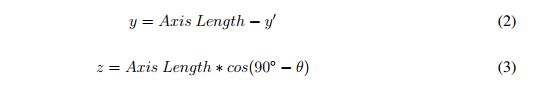
Point cloud registration, as implemented in this paper, is based on a geometric transformation in which the coordinate frame is located in the camera center when the camera is vertical. Also, it is important to clarify that the data to be registered is horizontally and vertically aligned. The vertical sweep that is obtained is controlled by the internal motor of the sensor using the library "Libfreenect" [28]. The program developed with this purpose grabs a point cloud every 10° , in the range [-30, 30°]. While the clouds are taken, the program transforms each one of these clouds to the coordinate frame considering that a displacement vector is generated because the origin of the rotation axis of the Kinect is not at the camera center. To calculate this vector, a geometric analysis is performed as shown in Figure 1.
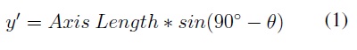
In Figure 1, the solid black line represents the profile silhouette of the sensor, and the dotted black line represents the sensor after vertical rotation at angle θ. Additionally, the dimension labeled as "z" is the z axis displacement, and the dimension labeled as "y" is the y axis displacement occurring when the sensor executes the rotation. Therefore:

Then, the transformation is executed according to the following matrix transformation:
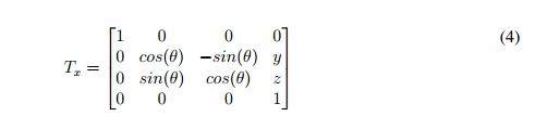
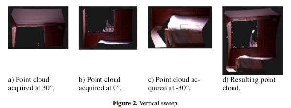
For instance, the resulting point cloud obtained through the transformation of the point clouds captured at 30° (Figure 2(a)and -30° (Figure 2(c)) to the coordinate frame at (0°) (Figure 2(b)). The registered cloud is shown in Figure 2(d).
Because the internal motor of the sensor does not allow the performance of horizontal sweeps, a simple structure that has markings at each 10° and that is rotated manually was designed for this purpose. When these rotations are made (being γ the rotation angle), there is no displacement vector; consequently, the matrix transformation used to perform this sweep is represented as follows:
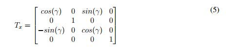
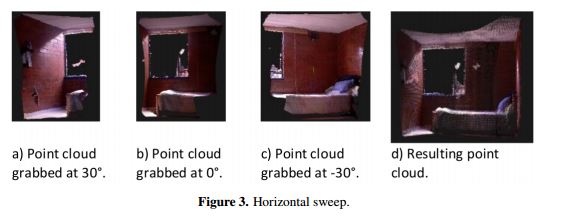
After this last transformation, the point clouds compose a single scene that is ready to be processed. Then, to summarize the process to obtain this single scene, the first step is to accomplish multiple vertical sweeps at different horizontal angles to obtain all desired views of the scene. At the same time, the vertical sweep is being performed, and the point clouds grabbed are being transformed using Equation 4. Then, with these clouds obtained from the vertical sweeps (Figure 3a-3c), a horizontal transformation is carried out by using Equation (5), to obtain a point cloud as show in Figure 3d.
3.Classification of basic structures
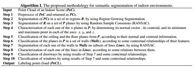
The classification is performed considering the position of each of the segments related to the coordinate frame of the point cloud and also considering the relationships among them. For instance, both ceiling and floor have their normal on the vertical axis, are parallel, and have the biggest and the smallest centroid position on that axis among all the other planes. The proposed methodology is presented in Algorithm I .
3.1 Preprocessing
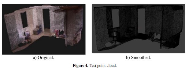
The point cloud pre-processing is carried out in three steps. First, we remove outliers. Second, we perform a VoxelGrid filtering in order to reduce the number of points to be analyzed [29]. Finally, to smooth and resample noisy data, a smoothing process based on Moving Least Squares (MLS) is used. This smoothing process uses a KDTree method to search and set a neighborhood within a determined radius; then, through MLS, normal vectors are calculated, and a polynomial high order interpolation is carried out [29]. Figure 4b shows a smoothed point cloud of the tested data depicted in Figure 4a.
3.2 Data segmention and feature extraction
After a point cloud is filtered, voxelized and smoothed, the following step is to segment the point cloud to find the boundaries of the objects or structures that integrate the 3D cloud. Cloud features are extracted and used to find the mentioned structures faster and separately.
3.2.1 Region Growing Segmentation
The Region Growing Segmentation (RGS) method is an algorithm that merges the points that are close enough in terms of the smoothness constraint [29].This method begins by designating a seed value to the point with minimum curvature (PCs0), in the evaluated neighborhood.The curvature κ is calculated as the rotation speed of the plane tangent (T) to the point ( κ = ||dT/ds ||). Then, the region A grows with the Pt point (A ← to the region A\ Pt) until there is an abrupt change (the symbol A\Pt means to add the point Pt to the region A)This abrupt change occurs when the curvature value of the analyzed point is less than the threshold value (κ (Pt) < Cth);this point is then added as a new seed (Sc ← Sc ∪ Pt), and the current seed is no longer one of these seeds. The process then starts again.
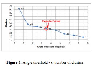
The threshold values of curvature and angle are defined empirically through experimentation. The definition of these values is very important to obtain a good performance from the method. The threshold values were varied to determine which values show the best results in the segmentation. The curvature threshold value was arbitrarily stated (the fixed value was 1.0), and the angle threshold was fitted over this curvature. For instance, the number of clusters that must be found by RGS for the point cloud in Figure 4a. is 33. Thus, according to the results depicted in Figure 5, the optimal value chosen for the angle threshold is 3.5°. These values are applicable to all the datasets because they were grabbed and processed in the same way.
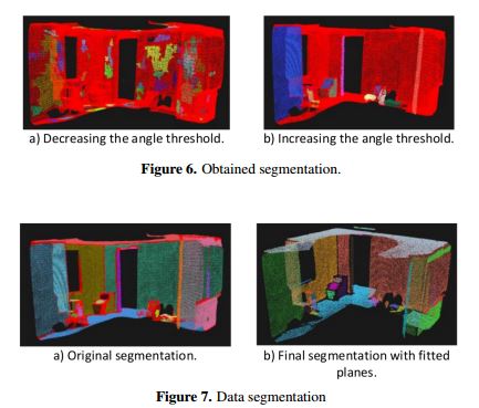
Figure 5 shows that when the angle threshold is reduced an over-segmentation occurs because the algorithm is more sensible (Figure 6a). When the angle threshold is increased, the majority of the points are not assigned to a segment (Figure 6b). All red points observed in Figure 6 are those points that are not clustered in a segment. With the appropriate threshold values, the resulting segmentation for the point cloud shown in Figure 4a. is the point cloud of Figure 7a. A total of 33 clusters were found.
3.2.2. Random Sample Consensus (RANSAC) plane segmentation
This method was selected because of the flatness of ceilings, floors and walls. The first proposal was created to segment the point clouds directly using RANSAC plane segmentation over the preprocessed cloud. However, as RANSAC method finds geometrical planes (planes extending to infinity), it can take points belonging to other planes due to the intersection that occurs among them. Furthermore, these planes are not very accurate and may be identified as a single plane, when there are actually two or three planes. For this reason, a solution was developed to combine this method with RGS.
We combined RANSAC with RGS instead of simply using RGS because RANSAC not only helps us to segment the regions that RGS kept mistakenly joined, but also helps us to obtain features of these segments by obtaining the plane coefficients that represent each one of them. RANSAC finds all the points that fit a plane based on distance criteria. When RANSAC attains to fit a set of points to the plane model, these coefficients correspond to the coefficients a, b, c, and d of the general equation of the plane (Equation(6)). The process is iterative and has a minimum amount of data to fit the model. Finally, when all points have been fitted to a model, a set of planes P is created, where P = pi and i = 1, . . . , n.

Every time a plane is found, the points that fit in the model are projected to this plane to improve the visualization of the model. The resulting point cloud is presented in Figure 7b. Each of the walls, floors, ceilings, and even planes of present objects inside the scene are segmented and identified with different colors. The resulting point cloud is cleaner due to the projection obtained.
3.2.3. Characterization of the planes
The classification of all the structures is accomplished based on contextual relationships and their position related to the coordinate frame. For instance, both floor and ceiling have their normals in the y axis and walls are orthogonal to them (Manhattan structure). Therefore, finding the normal vector of each one of the segments is important for the classification step. Additionally, location and size planes help to determine if they are just part of the objects inside the scene or if they are the structures that we are looking for.
Hence, the features used are as follows: i) Coefficients a, b, and c for each one of the n planes
found through the RANSAC plane segmentation (according to eq. (6)). Where a, b, and c are the
normals of the plane  . ii) Centroid of each one of the
n planes, where cx is the centroid of a plane in the x axis, cy in the y axis, and cz in the z axis:
. ii) Centroid of each one of the
n planes, where cx is the centroid of a plane in the x axis, cy in the y axis, and cz in the z axis:
 .Maximum and minimum points of the planes in each axis of the coordinate
system.
.Maximum and minimum points of the planes in each axis of the coordinate
system.  is the vector of the minimum points, and
  is the vector of the maximum points:
 and
and  .
.
3.3. Floor and ceiling classification
Due to the position in which the reference system of the scenes is located, the classification of floor and ceiling is carried out using the normal and centroid information. Both ceilings and floors, as stated above, have their normal on the y axis, and their centroids on this axis are the lowest and the highest among all the others, correspondingly. Therefore, those planes obtained by using RANSAC, that meet these conditions are labeled as ceiling and floor, respectively.
3.4. Wall classification
To classify and label certain planes, such as walls, the features used were contextual features, where it was assumed that they are always orthogonal to the floor and to the ceiling and that they have contact with both the floor and ceiling (Manhattan indoor structure [10]). A contact threshold of 10cm is established. This threshold is created because when the RGS is applied, it is not possible to cluster the borders of each one of the planes accurately. Therefore, the borders are not assigned to any cluster, and a small distance between the floor and walls, and between the ceiling and walls is generated.
After identifying some walls and occlusions, the walls are grouped based on their location and position with respect to the coordinate frame. All walls with their normal on the x axis and their centroid located at the positive side of this axis are grouped and counted. In the same way, all walls that have their normal in x as well and have their centroid located on the negative side of the x axis are grouped. The same procedure is carried out with walls that have their normal on the z axis; they are grouped depending on the side where their centroid is located, and the number of walls classified in these groups is counted. This clustering allows us to identify whether there is a wall that was not labeled as a wall because it is not possible to identify an occlusion on a side where there is not a wall. Therefore, if an occlusion is found on a side where there is no wall, it is probable that this occlusion is really a wall, its label is changed, and it is classified as a wall. In this way, the number of walls increases.
When all the walls have been identified, the next step is to project into the walls all the remaining occlusions to avoid future non-existent holes in walls that can later generate wrong classifications. In addition, due to fact that the RGS method classifies as different planes those that are totally divided by a hole generated, for example, by an opened door, an algorithm that clusters these types of walls into a single wall is created. Thus, the number of walls can be reduced.
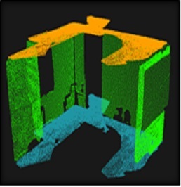
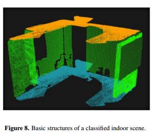
The semantics used to represent the structures classified are as follows: walls are represented in green, floors in blue and ceilings in orange. The classification result is shown in Figure 8.
4. Doorway and window classification
To reduce the classification time for doors and windows, this process is carried out after labeling the basic structures. If walls are labeled, the searching for doors and windows can be performed in fewer planes because the doors and windows will only be located in the walls. It is important to highlight that only open doors or doors at a different level of the wall will be classified.
4.1. Wall segmentation
In finding and labeling doorways and windows, only the planes labeled as walls are segmented. By means of contextual relationships, doorways and windows are not commonly known to be located in ceilings and floors. Because the Kinect has an infrared sensor to measure depth and glass is not able to reflect the infrared spectrum, the windows in indoor scenes are not acquired. In this way, both windows and doorways are observed as holes in the walls. Therefore, the challenge results in finding holes that can be doorways or windows.
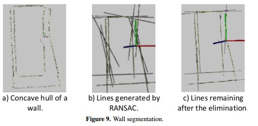
Before starting with the segmentation process, the borders of the walls were found by calculating each one of their concave hulls and then applying the RANSAC line segmentation method. A large quantity of lines is obtained, and the lines that do not describe the borders accurately are to be eliminated. For instance, if the concave hull of a wall contains the points shown in Figure 9a, the segmentation obtained is the one shown in Figure 9b. It is, therefore, necessary to eliminate all those lines that are not parallel or orthogonal to the floor.
The elimination process is accomplished by finding the angle between each one of the lines and the normal of the floor. If the angle is different from 0°, 90°, 180°, or 270°, with a permissible deviation, the line is eliminated (Figure 9c).
Furthermore, all the lines that represent the intersection between two planes (two walls), are added to this set of lines, to ensure the possibility of finding doors that are not contained in a plane but are on the border of a plane. The only condition is that in order to add these lines to the found set, they must have contact with points of the cloud in a maximum radius of 10 cm, because we might have a scene that was not grabbed at 360° or a scene in which the indoor geometry does not have a quadrangular shape (Manhattan assumption). The radius of 10 cm is fixed because, even if the shape of the room is quadrangular, there is a distance between planes generated by the RGS process, as was already explained.
RANSAC lines often find two or more lines that describe the same segment, something that is not practical because it can generate over-segmentation of the regions. For this reason, lines that are very close to each other are also eliminated, obtaining a total of nl number of lines.
4.2. Characterization of segmented walls
All remaining lines are intersected with each other. These intersections are used to define the
distance between two parallel lines; for instance, to measure the gap between two parallel lines,
the intersection points that they have with a common line are taken and compared by measuring the
distance between them. This measure is also the distance between both lines. The features taken
into account for both doorways and windows were as follows: i) The distance between parallel
lines that describe the width of the doorway or the window. If a wall has its normal on the x axis:
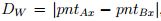 , where pntAx is the point on the x axis in which the line A intersects a
line C, and pntBx is the point on the x axis in which the line B intersects a line C. If a wall has its
normal on the z axis:
, where pntAx is the point on the x axis in which the line A intersects a
line C, and pntBx is the point on the x axis in which the line B intersects a line C. If a wall has its
normal on the z axis: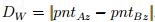 , where pntAz is the point on the z axis in which the
line A intersects a line C, and pntBz is the point on the z axis in which the line B intersects a line
C. ii) The distance between parallel lines that describe the height of the doorway or the window:
, where pntAz is the point on the z axis in which the
line A intersects a line C, and pntBz is the point on the z axis in which the line B intersects a line
C. ii) The distance between parallel lines that describe the height of the doorway or the window:
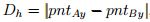 , where pntAy is the point on the y axis in which the line A intersects a line
C, and pntBy is the point on the y axis in which the line B intersects a line C. iii) The number of
points inside each one of the rectangles. An additional feature used for window classification was:
Position of the upper rectangle edge on the y axis: Pos= pnty , where pnty is a point on the y axis
belonging to a line of the upper edge of a rectangle.
, where pntAy is the point on the y axis in which the line A intersects a line
C, and pntBy is the point on the y axis in which the line B intersects a line C. iii) The number of
points inside each one of the rectangles. An additional feature used for window classification was:
Position of the upper rectangle edge on the y axis: Pos= pnty , where pnty is a point on the y axis
belonging to a line of the upper edge of a rectangle.
4.3. Doorway classification
To create some rectangles and classify them as doorways, the features found were used considering contextual relationships and common features among common doorways. Regularly, in common indoor scenes, doorways have a minimum height of 1.8 m and a maximum height of 2.3 m (1.8 ≤Dh ≤ 2.3). In the same way, doorways have a minimum width of 0.6 m and a maximum width of 1 m (0.6 ≤ Dw ≤ 1). For these reasons, all pairs of lines that have these distances between them are mixed to create rectangles that are saved as those that describe possible doorways.
The last step to classify these rectangles is to count each one of their inside points. Ideally, a rectangle that represents a doorway should not have points inside, but because the lines found do not accurately describe the edge of the point cloud, a threshold of 15% is defined. Therefore, a rectangle that has less than 15% of its area full of points is classified as a doorway. These rectangles are saved in a matrix called Door with size nd.
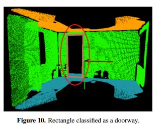
Sometimes, the process results in various representations for a single doorway. To solve this problem, a grouping is carried out by considering the following parameters: area, number of vertical lines in common, and percentage of area full of points. In this way, all the nd rectangles are analyzed by pairs. If the rectangles have a line in common or one of them is inside the other, the rectangle with the greatest percentage of points inside is eliminated as a doorway, and the number nd is decreased. In the case of the point cloud shown in Figure 4a, the doorway classification gives as a result the point cloud shown in Figure 10. The brown lines are the semantics used to show a doorway, and a red circle is added to highlight the doorway.
4.4. Window classification
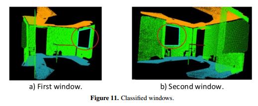
Similar to the doorway classification process, to create some rectangles and classify them as windows, window size restrictions and position restrictions are defined. In the case of windows, there is not a maximum size restriction but there is a minimum size restriction. A common window has a minimum height and width of 0.3 m, where Dh ≤ 0.3, and Dw ≤ 0.3, and their upper edge is always above the centroid in the y axis of the wall: Pos < cywall. All pairs of lines that meet these features are combined to create rectangles that are saved as if describing possible windows. The condition Pos cywall is established because in a common indoor scene, a window always has its upper edge nearer to the ceiling than to the floor. Otherwise, the rectangle could be a result of an occlusion. As in doorway classification, a counting of points inside each one of the rectangles is also performed, and the percentage allowed is the same. The only step previous to classifying a rectangle as a window is to check that none of the lateral lines of this rectangle belongs to another rectangle classified as a doorway. With the selected rectangles, the clustering is executed following the same principles as door clustering. Figure 11 shows the windows obtained for data in Figure 4a.
Results
Tests were performed using a 2.6 GHz Intel Core 2 Duo processor computer with 4GB RAM, running an Ubuntu 12.10 operating system. The sensor used to grab the point clouds was a Microsoft Kinect Sensor for XBOX 360. The libraries used were Libfreenect for Kinect’s hardware handling, Point Cloud Library PCL 1.7 for point cloud processing [30], Eigen 3.2.0 and OpenCV libraries for matrix and vector operations, and the Visualization Toolkit VTK 5.8 for image visualization.
The initial sensor position relative to the environment is at 0°, both horizontally and vertically, so that the sensor is facing a wall at a 90° angle. Furthermore, the Kinect is located approximately at mid-height of the scene to ensure that both floor and ceiling are captured. The system could be mounted in a mobile robot, a Robotino for example, to improve the data acquisition and enlarge its application.
The algorithm was tested in 24 scenes which contained 24 floors, 24 ceilings, 90 walls, 28 doorways and 20 windows. The global process applied after the data collection is: i) Pre-process the Point Cloud; ii) Segment the pre-processed Point Cloud; iii) Characterize each one of the segments obtained in Step ; iv) Classify the ceiling and floor; v) Classify the walls; vi) Segment the walls; vii) Characterize the wall segments; and viii) Classify doors and windows.
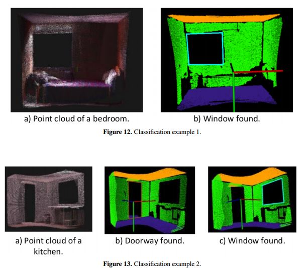
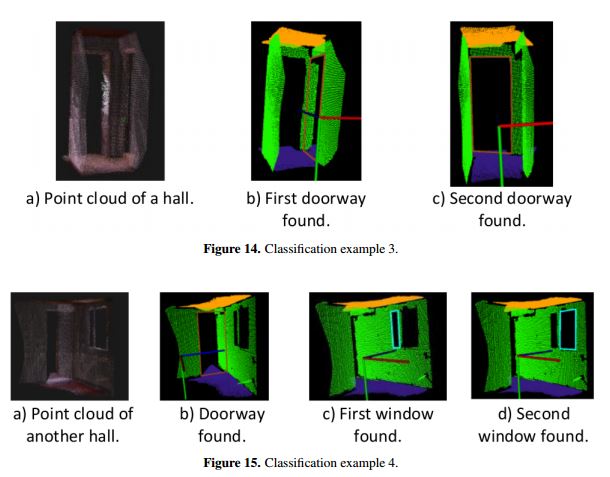
Some classifications that were carried out are shown in Figure 12-15. Figure 12 is the point cloud of a bedroom that has one window on a wall that is occluded by a bed. Figure 13 is a kitchen with one doorway and one window; the wall of the window is also occluded. Figure 14 is the image of a hall with two doorways. Figure 15 is another hall that has one doorway and one window divided by a window frame; this is why the algorithm identifies two windows.
After developing the tests by using each one of the 24 scenes, the results obtained are shown as a confusion matrix (Table I), where a complete success in elements such as ceilings and floors was achieved. Notation in Table I is: Doorways (Dw), Windows (Wd), Walls (Ws), Ceilings (C), Floors (F), and Not classified (NC).
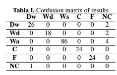
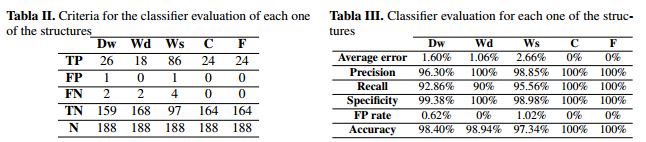
The information registered in Table I is represented as True Positive (TP), False Positive (FP), True Negative (TN), and False Negative (FN) results, obtaining a total element number (N). These results are provided in Table II. Then, this information is used to evaluate the classifier (see Table III). The evaluated aspects are as follows: i) Average error, the proportion of misclassification; ii) Precision, the proportion of cases that were correctly accepted; iii) Recall or Sensitivity, the proportion of true acceptance or the proportion of true positive elements; iv) Specificity, the proportion of true rejection or the proportion of true negative elements; v) False positive rate, the proportion of false acceptance; and vi) Accuracy, the accuracy of the classifier.
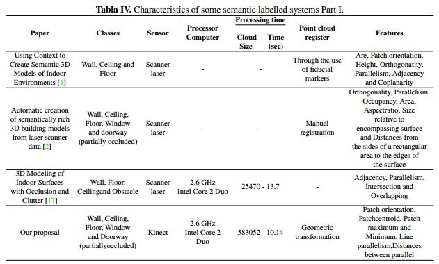
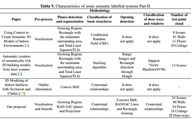
As mentioned above, the best results were obtained with ceilings and floors, reaching a precision of 100%, although the results obtained for the other structures were also satisfactory. In this way, when averaging of the algorithm performance, a precision of 99.03% and a recall of 95.68% were obtained. To give a qualitative idea of where the proposed method is located in relation to similar works, Tables IV and V are presented, which illustrate different characteristics of the proposed methodology.
Because the classification was based on the contextual relationships among the structures with Manhattan assumption [10], errors found were due to: noise, scenes that have walls that are not orthogonal; and an incorrect data collection. Taking into account all these errors, their source, and the features that the scenes need to fulfill to be correctly identified, it is projected to extend the types of indoor scenes to be labeled in future work. It is possible to fit the algorithm to identify all the environments in which the ceiling is not parallel to the floor. This identification would be possible by eliminating the condition that the ceiling has its normal vector on the y axis and by adding both its centroid on the y axis and its minimum on the y axis, which are the smallest among the features of the other planes. Additionally, the projection of occlusions can be improved if they are projected in the point in which an imaginary ray from the sensor intersects with the planes identified as walls. Finally, the labeling of other objects is possible if all of those that were not labeled and that have some relationships among them are analyzed. For instance, planes parallel to the floor that are not labeled as ceilings can be the top of a table under some contextual relationships.
The proposed system is designed to classify and label walls, ceilings, floors, doorways with open doors, doorways with closed doors recessed into walls, and partially occluded windows. However, there may be scenarios with doors to the level of the wall, curtained windows or glass walls. The system should be modified to have proper operation in such cases. In the first two cases, because the depth of objects does not change, i.e. the door or curtain are considered to be at the same level of the wall, but there is a change in texture or color, the modification would be to incorporate to the system color or texture descriptors, obtained from the image analysis. To deal with situations with glass walls, given that this material has properties of non Lambertian reflectance, the reconstruction technique of the scene should be modified. In [31] some of these reconstruction techniques are reviewed.
6. Conclusions
This paper presents a new method for semantic labeling of indoor scenes. The methodology that has been presented assumes a Manhattan indoor structure and is based mostly on contextual relationships among the objects, such as parallelism, orthogonality, window and doorway position related to the walls, and usual heights and widths of windows and doorways. The classification and labeling were performed without the need for a classifier that requires both training and a large amount data for that purpose. They were performed with contextual rules that allow an easy understanding of the process and also an identification of the reasons why there are some errors in labeling.
Furthermore, the data were captured with a low-cost sensor with a low resolution, and the computer employed to perform the tests has a processor that is below the standard. Although the algorithm can be tied to the way in which the data were collected, both the accuracy of labeling and processing time are satisfactory, and the computational requirements are closer to real time.
The next step is to continue with the improvement of this system. Firstly, making it less dependent on data collection and enlarging the objects or structures that can be identified, and particularly expanding the structures of indoor environments to structures that do not meet the Manhattan assumption. Secondly, assembling the acquisition system in a mobile robot.
References
[1] Xuehan Xiong and Daniel Huber, Using Context to Create Semantic 3D Model of Indoor Environments. Proceedings of the British Machine Vision Conference, 2010, pp. 1-11.
[2] Xuehan Xiong, Antonio Adan, Burcu Akinci and Daniel Huber, Automatic creation of semantically rich 3D building models from laser scanner data. Automation in Construction, Volume 31, May, 2013, pp. 325-337.
[3] Lei Shi, Sarath Kodagoda and Ravindra Ranasinghe, Fast indoor scene classification using 3D point clouds, Proceedings of Australasian Conference on Robotics and Automation (ACRA), 2011.
[4] Lei Shi, Sarath Kodagoda and Gamini Dissanayake, Laser range data based semantic labeling of places, International Conference on Intelligent Robots and Systems (IEEE/RSJ), 2010, pp. 5941-5946.
[5] Radu Rusu, Zoltan Marton, Nico Blodow, Andreas Holzbach and Michael Beetz, Model-based and learned semantic object labeling in 3D point cloud maps of kitchen environments. IEEE/RSJ International Conference on Intelligent Robots and Systems (IROS), 2009, pp. 3601-3608.
[6] Leydy Muñoz, Edilson Quiñonez y Héctor Victoria, Reconstrucción 3D de objetos sumergidos en aguas limpias. Ingeniería, Vol. 18, N0. 2, pp.36-53.
[7] Julien Valentin, Vibhav Vineet, Ming Cheng, David Kim, Jaime Shotton, Pushmeet Kohli, Matthias Niessner, Antonio Criminisi, Shahram Izadi and Philip Torr, SemanticPaint: Interactive 3D Labeling and Learning at your Fingertips. ACM Transactions on Graphics, Volume 34, Number 5, 2015.
[8] Seong Park and Ki Hong, Recovering an indoor 3D layout with top-down semantic segmentation from a single image. Pattern Recognition Letters, Volume 68, Part 1, December 2015, pp. 70-75.
[9] Sid Bao, Axel Furlan, Li Fei and Silvio Savarese, Understanding the 3D layout of a cluttered room from multiple images. 2014 IEEE Winter Conference on Applications of Computer Vision (WACV), 2014, pp. 690-697.
[10] Alex Flint, David Murray and Ian Reid, Manhattan scene understanding using monocular, stereo, and 3d features. 2011 International Conference on Computer Vision, 2011, pp. 2228-2235.
[11] Erick Delage, Honglak Lee and Andrew Ng, A dynamic bayesian network model for autonomous 3D reconstruction from a single indoor image. Proceedings of the 2006 IEEE Conference on Computer Vision and Pattern Recognition, 2006, pp. 2418-2428.
[12] ] Shi Wenxia and J. Samarabandu, Investigating the performance of corridor and door detection algorithms in different environments. Proceedings of the International Conference on Information and Automation, 2006, pp. 206-211.
[13] Ru0 Zhang, Ping Tsai, James Cryer and Mubarak Shah, Shape-from shading: a survey. IEEE Transactions on Pattern Analysis and Machine Intelligence, Volume 21, Number 8, 1999, pp. 690-706.
[14] Hao Wu, Guo Tian, Yan Li, Feng Zhou and Peng Duan, Spatial semantic hybrid map building and application of mobile service robot. Robotics and Autonomous Systems, Volume 62, Number 6, 2014, pp. 923-941.
[15] Pooja Viswanathan, David Meger, Tristram Southey, James Little and Alan Mackworth, Automated spatialsemantic modeling with applications to place labeling and informed search. Proceedings of the Canadian Conference on Computer and Robot Vision, 2009, pp. 284-291.
[16] Angela Budroni and Jan Bohm, Automatic 3D modelling of indoor manhattan-world scenes from laser data.Proceedings of the International Archives of Photogrammetry, Remote Sensing and Spatial Information Sciences, 2010, pp. 115-120.
[17] S.A. Abdul-Shukor, K.W. Young and E. Rushforth, 3D Modeling of Indoor Surfaces with Occlusion and Clutter. Proceedings of the 2011 IEEE International Conference on Mechatronics, 2011, pp. 282-287.
[18] Martin Weinmann, Boris Jutzi, Stefan Hinz and Clement Mallet, Semantic point cloud interpretation based on optimal neighbor- hoods, relevant features and efficient classifiers. ISPRS Journal of Photogrammetry and Remote Sensing, Volume 105, 2015, pp. 286-304.
[19] Andrés Serna and Beatriz Marcotegui, Detection, segmentation and classification of 3D urban objects using mathematical mor- phology and supervised learning. ISPRS Journal of Photogrammetry and Remote Sensing, Volume 93, 2014, pp. 243-255.
[20] Microsoft, Kinect, February 2015, [On line], Available on http://www.xbox.com/en-us/kinect.
[21] Hema Koppula, Abhishek Anand, Thorsten Joachims and Ashutosh Saxena, Semantic labeling of 3D point clouds for indoor scenes. Proceedings of the Advances in Neural Information Processing Systems, 2011, pp. 1-9.
[22] Xiaofeng Ren, Liefeng Bo, and Dieter Fox, RGB-(D) scene labeling: Features and algorithm. Proceedings of the 2012 IEEE International Conference on Computer Vision and Pattern Recognition, 2012, pp. 2759-2766.
[23] Paul Besl and Neil McKay, A method for registration of 3-D shapes, IEEE Transactions on Pattern Analysis and Machine Intelligence, Volume 14, Number 2, 1992, pp. 239-256.
[24] Óscar Mozos, Cyrill Stachniss and Wolfram Burgard. Supervised learning of places from range data using adaboost. Proceedings of the 2005 IEEE International Conference on Robotics and Automation, 2005, pp. 1730-1735.
[25] Andreas Nuchter and Joachim Hertzberg, Towards semantic maps for mobile robots. Robotics and Autonomous Systems, Volume 56, Number 11, 2008, pp. 915-926.
[26] Alex Flint, Christopher Mei, David Murray and Ian Reid, A dynamic programming approach to reconstructing building interiors. Proceedings of the 13th IEEE European Conference on Computer Vision, 2010, pp. 394-407.
[27] Martin Fischler and Robert Bolles, Random Sample Consensus: A Paradigm for Model Fitting with Applications to Image Analysis and Automated Cartography. Communications of the ACM, Volume 24, Number 6, 1981, pp.381-395.
[28] Open Kinect Project, Open Kinect, July 2015, [On line], Available on: http://openkinect.org/wiki/Main Page .
[29] Point Cloud Library, Documentation, March 2015, [On line], Available on: http://pointclouds.org/documentation/tutorials/.
[30] Point Cloud Library, What is it?, September 2015, [On line], Available on: http://pointclouds.org/.
[31] Ivo Ihrke, Kiriakos N. Kutulakos, Hendrik P. A. Lensch, Marcus Magnor and Wolfgang Heidrich, Transparent and Specular Object Reconstruction. Computer Graphics Forum. Volume 29, Number 8, 2010, pp. 2400-2426.
License
![]()
From the edition of the V23N3 of year 2018 forward, the Creative Commons License "Attribution-Non-Commercial - No Derivative Works " is changed to the following:
Attribution - Non-Commercial - Share the same: this license allows others to distribute, remix, retouch, and create from your work in a non-commercial way, as long as they give you credit and license their new creations under the same conditions.

2.jpg)