
DOI:
https://doi.org/10.14483/23448350.15797Published:
05/01/2020Issue:
Vol. 38 No. 2 (2020): May-August 2020Section:
Science and EngineeringEstimating Market Expectations for Portfolio Selection Using Penalized Statistical Models
Estimación de expectativas del mercado para la selección de portafolios usando modelos estadísticos penalizados
Keywords:
Penalized models, regularization, state price density estimation, financial options, portfolio optimization (en).Keywords:
Optimización de portafolios, regularización, modelos penalizados, estimación de la densidad del precio implícita, opciones financieras (es).Downloads
References
Aït-Sahalia, Y., & Lo, A. W. (1998). Nonparametric Estimation of State-Price Densities Implicit in Financial Asset Prices. The Journal of Finance, 53(2), 499–547. https://doi.org/10.1111/0022-1082.215228
Aït-Sahalia, Y., &Duarte, J. (2003). Nonparametric Option Pricing under Shape Restrictions. Journal of Econometrics, 116(1-2), 9–47. https://doi.org/10.1016/S0304-4076(03)00102-7
Black, F., & Scholes, M. (1973). The Pricing of Options and Corporate Liabilities. The Journal of Political Economy, 81(3), 637–654. https://doi.org/10.1086/260062
Bondarenko, O. (2003). Estimation of Risk-Neutral Densities Using Positive Convolution Approximation. Journal of Econometrics, 116(1-2), 85–112. https://doi.org/10.1016/S0304-4076(03)00104-0
Breeden, D. T., & Litzenberger, R. H. (1978). Prices of State-Contingent Claims Implicit in Option Prices. The Journal of Business, 51(4), 621–651. https://doi.org/10.1086/296025
DeMiguel, V., Garlapi, L., & Uppal, R. (2009a). Optimal Versus Naive Diversification: How Ineficient Is the 1/N Portfolio Strategy?. The Review of Financial Studies, 22(5), 1915–1953. https://doi.org/10.1093/rfs/hhm075
DeMiguel, V., Garlappi, L., Nogales, F. J., & Uppal, R. (2009b). A Generalized Approach to Portfolio Optimization: Improving Performance by Constraining Portfolio Norms. Management Science, 55(5), 798–812. https://doi.org/10.1287/mnsc.1080.0986
DeMiguel, V., Plyakha, Y., Uppal, R., & Vilkov, G. (2013). Improving Portfolio Selection Using Option-Implied Volatility and Skewness. Journal of Financial and Quantitative Analysis, 48(6), 1813–1845. https://doi.org/10.1017/S0022109013000616
Fan, J., Zhang, J., & Yu, K. (2012). Vast Portfolio Selection with Gross-Exposure Constraints. Journal of the American Statistical Association, 107(498), 592–606. https://doi.org/10.1080/01621459.2012.682825
Jagannathan, R., & Ma, T. (2003). Risk Reduction in Large Portfolios: Why Imposing the Wrong Constraints Helps. The Journal of Finance, 58(4), 1651–1684. https://doi.org/10.1111/1540-6261.00580
Jorion, P. (1986). Bayes-Stein Estimation for Portfolio Analysis. Journal of Financial and Quantitative Analysis, 21(3), 279–292. https://doi.org/10.2307/2331042
Jorion, P. (2007). “Value at Risk - The New Benchmark for Managing Financial Risk”. (3rd ed.). The McGraw Hill Companies, Inc.
Kan, R., & Zhou, G. (2007). Optimal Portfolio Choice with Parameter Uncertainty. The Journal of Financial and Quantitative Analysis, 42(3): 621–656. https://doi.org/10.1017/S0022109000004129
Ledoit, O., & Wolf, M. (2003). Improved Estimation of the Covariance Matrix of Stock Returns With an Application to Portfolio Selection. Journal of Empirical Finance, 10(5), 603–621. https://doi.org/10.1016/S0927-5398(03)00007-0
Ledoit, O., & Wolf, M. (2004). Honey, I Shrunk the Sample Covariance Matrix. Journal of Portfolio Management, 30(4), 110–119. https://doi.org/10.3905/jpm.2004.110
Li, J. (2015). Sparse and Stable Portfolio Selection With Parameter Uncertainty. Journal of Business & Economic Statistics, 33(3), 381–392. https://doi.org/10.1080/07350015.2014.954708
Ludwig, M. (2015). Robust Estimation of Shape-Constrained State Price Density Surfaces. The Journal of Derivatives, 22(3), 56–72. https://doi.org/10.3905/jod.2015.22.3.056
Lwin, K. T., Qu, R., & MacCarthy, B. L. (2017). Mean-VaR Portfolio Optimization: A Nonparametric Approach. European Journal of Operational Research, 260(2), 751–766. https://doi.org/10.1016/j.ejor.2017.01.005
Markowitz, H. (1952). Portfolio Selection. The Journal of Finance, 7(1), 77–91. https://doi.org/10.1111/j.1540-6261.1952.tb01525.x
Markowitz, H. (1959). Portfolio Selection: Efficient Diversification of Investments. New York: John Willey and Sons.
Morgan, J. P. (1996). RiskMetrics (TM): Technical Document. Morgan Guaranty Trust Company.
Peterson, B. G., Carl, P., Boudt, K., Bennett, R., Ulrich, J., Zivot, E., … & Wuertz, D. (2018). Econometric Tools for Performance and Risk Analysis (version 1.5.2). R.
Shen, W., Wang, J., & Ma, S. (2014). Doubly Regularized Portfolio with Risk Minimization. In, Proceedings of the Twenty-Eighth AAAI Conference on Artificial Intelligence (pp. 1286-1292). AAAI Press.
Yatchew, A., & Härdle, W. (2006). Nonparametric State Price Densisty Estimation Using Constrained Least Squares and the Bootstrap. Journal of Econometrics, 133(2), 579–599. https://doi.org/10.1016/j.jeconom.2005.06.031
Young, T. W. (1991). Calmar Ratio: A Smoother Tool. Futures Magazine, 20(1), 40.
Yuan, M. (2009). State Price Density Estimation via Nonparametric Mixtures. The Annals of Applied Statistics, 3(3), 963–984. https://doi.org/10.1214/09-AOAS246
How to Cite
APA
ACM
ACS
ABNT
Chicago
Harvard
IEEE
MLA
Turabian
Vancouver
Download Citation
Recibido: de enero de 2020; Aceptado: de abril de 2020
Abstract
The portfolio selection problem can be viewed as an optimization problem that maximizes the risk-return relationship. It consists of a number of elements, such as an objective function, decision variables and input parameters, which are used to predict expected returns and the covariance between the said returns. However, the real values of these parameters cannot be directly observed; thus, estimations based on historical data are required. Historical data, however, can often result in modelling errors when the parameters are replaced by their estimations. We propose to address this by using some regularization mechanisms in the optimization. In addition, we explore the use of implicit information to improve the portfolio performance, such as options market prices, which are a rich source of investor expectations. Accordingly, we propose a new estimator for risk and return that combines historical and implicit information in the portfolio selection problem. We implement the new estimators for the mean-VAR and mean-VaR2 problems using an elastic-net model that reduces the risk of all estimations performed. The results suggest that the model has a good out-of-sample performance that is superior to models with pure historical estimations.
Keywords:
Penalized models, portfolio optimization, regularization, state price density estimation, financial options..Resumen
El problema de selección de portafolios puede ser visto como un problema de optimización que maximiza una relación riesgo-retorno cuyos parámetros son los retornos esperados y las covarianzas entre ellos. Sin embargo, los valores reales de dichos parámetros no son observables, por lo cual es necesario realizar estimaciones que comúnmente están basadas en datos históricos. Estas estimaciones pueden introducir errores en el modelo, haciendo necesario usar diferentes mecanismos de regularización, como los propuestos en el presente estudio. Además, proponemos el uso de información adicional para mejorar el desempeño de los portafolios, como los son los precios de las opciones que contienen una rica fuente de información que muestra las expectativas de los inversionistas con base en sus conocimientos acerca de cada uno de los subyacentes. De esta manera, proponemos el uso de un nuevo estimador de riesgo-retorno que mezcla la información histórica con la implícita para el problema de selección de portafolios. Implementamos los nuevos estimadores para el problema de Media-Varianza y Media-VaR2 a través de un modelo de red-elástica que permite reducir el impacto del riesgo de las estimaciones realizadas. Los resultados sugieren rendimientos de portafolio superiores a los modelos con estimadores basados en datos históricos.
Palabras clave:
Optimización de portafolios, regularización, modelos penalizados, estimación de la densidad del precio implícita, opciones financieras..Resumo
O problema de seleção de portfólio pode ser visto como um problema de otimização que maximiza uma taxa de risco-retorno. Em seguida, possui uma função objetiva, variáveis de decisão e parâmetros: retornos esperados e covariância entre eles. Os valores reais desses parâmetros são desconhecidos para nós, portanto, devemos fazer estimativas que geralmente são baseadas em dados históricos. Além do erro envolvido na estimativa, devemos reconhecer que os dados históricos não são os únicos que poderíamos usar. Os preços das opções são uma rica fonte de informações que mostra as expectativas dos investidores com base em seus conhecimentos sobre cada um dos subjacentes. Dessa forma, propomos o uso de um novo estimador de risco-retorno que mescla informações históricas e implícitas para o problema de seleção de portfólio. Implementamos os novos estimadores para o problema de Media-Variance e Media-VaR2 por meio de um modelo elástico de rede que permite reduzir o impacto no risco das estimativas feitas.
Palavras-chaves:
Otimização de portfólio, regularização, modelos estatísticos penalizados, estimativa implícita da densidade de preços, opções financeiras.Introduction
According to Harry Markowitz (1952, 1959), an investor builds a portfolio by selecting a group of assets and choosing the weight held by each one, motivated not only by risk minimization and return maximization but also by risk diversification. Although Markowitz created a framework to understand asset selection, it is insufficient because it does not consider parameter’s uncertainty; that is, it does not consider the uncertainty of expected asset returns nor of the covariance between them. Unfortunately, for stock market predictions, the real values of parameters are not achievable, so we must rely on estimations. As a naïve solution, the optimization problem can be solved by combining the expected return and the covariance matrix based on historical data. However, this solution does not result in good out-of-sample performance (Kan and Zhou, 2007) and some adjustments are needed to improve it.
In the existing literature, shrinkage estimators have been proposed (Ledoit and Wolf, 2003, 2004; Jorion, 1986), which correct the parameters before the optimization problem, thereby reducing estimation error. Alternatively, creating constraints over the portfolio weights, thereby shrinking them, can also reduce estimation errors (DeMiguel et al., 2009a; DeMiguel et al., 2009b; Jagannathan and Ma, 2003). In essence, imposing constraints over the L1 and L2 norms of the vector of portfolio weights using linear regression (elastic net) results in risk reduction and an improved out-of-sample portfolio performance (Li, 2015). The aforementioned studies depend on historical prices to perform estimations. Although historical prices are widely available, other sources exist for market estimation. A fully developed options market, for instance, is a rich source of investor expectations with respect to the price fluctuations of assets. Indeed, information from the options market has been used to price exotic derivatives, assess market beliefs, examine market rationality, estimate the risk preferences of investors, and manage risk (Bondarenko, 2003).
In this study, we combine historical prices with data from the options market, implicit information, to estimate the return vector and covariance matrix. Implicit information is summarized in the state price density (SPD) (Aït-Sahalia and Lo, 1998); by gaining access to the SPD of each asset in our portfolio, we can estimate their expected return and variance, thereby obtaining the inputs to solve the portfolio selection problem. We construct a portfolio using a set of options with the maturity dates τ days forward and, τ days later we rebalance the portfolio. To do this, we use Li’s (2015) elastic net. Moreover, since we estimate the full SPD, we use other risk measurements for the optimization problem, such as value at risk (VaR) (Morgan, 1996). This measure is widely used owing to its several advantages; most importantly, it provides information on investor underperformance, not on both underperformance and overperformance as variance (Lwin et al., 2017), which means it is easier to interpret. Accordingly, in this study, we solve the traditional Mean-VAR bi-objective problem and motivated by the advantages of VaR, we solve a modified portfolio selection problem mean-VaR2 using an elastic-net model and the proposed historical-implicit estimators.
Methodology
We know that each investor has a portfolio with an expected return of
 with risk over their investment of
 , where denotes a column vector of p weights (one for each asset), µ denotes a column vector with the expected return of each asset, and Σ denotes the
 variance-covariance matrix. Accordingly, the risk-return relationship that is maximized can be expressed as follows:
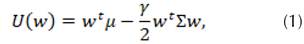
where
 is a risk aversion coefficient. The optimal value of can be found when

According to Li (2015) , the ordinary least squares (OLS) estimator of the linear regression model,
 can be obtained by minimizing
  ,that is, when
 . Comparing this equation with the one obtained after deriving (16) with respect to , it is evident that both are of the form
 ; therefore, we can compare the coefficients to obtain the following:

Since Σ is a positive semi-definite matrix, it can be expressed as
 .Accordingly,
 can be estimated. Taking this into account, from
 , we obtain the following:

and from
 , we obtain the following:

Therefore, by applying these definitions of X and Y, the portfolio selection problem can be solved using the OLS estimator of the linear regression problem

Improvements to the linear regression estimators
The linear regression model is restricted due to its assumptions. For instance, if the variables,
 and
and
 , are highly correlated, the estimators, and , will not result in adequate conclusions. To address this, we can shrink the linear regression estimators, thereby correcting them. The elastic-net model presented in (4) solves the linear regression model but creating constraints over the L1 and L2 norms of the vector of coefficients, thereby shrinking it:

Indeed, this model will help correct a number of elements. First of all, an inevitable correlation exists between stock market assets, which means that a basic linear regression model will discard important information on highly correlated variables. By applying the elastic-net model, we can regulate the portfolio weights of similar assets. In other words, the elastic-net model reduces the risk of our estimations by reducing the uncertainty of the expected returns, the covariance matrix, and its inverse. In addition, the correlation between assets results in an ill-conditioned covariance matrix. To address this problem, the diagonal elements of the matrix,
 , should be increased by a constant value. Moreover, by creating the term,
 , in the elastic-net model, we can improve the estimation of
 (Li, 2015). According to Shen, Wang, and Ma (2014) , this L2 constraint ensures that portfolio weights are similar under rebalancing for consecutive investment periods, thereby reducing transaction costs. Alternatively, if we measure the estimation risk as the difference between (1) evaluated with real parameters versus estimated parameters; i.e.
 , this calculation is regulated by the L1 norm of the vector of coefficients with the following expression:

Therefore, creating a constraint over the L1 norm reduces the estimation risk of μ and ? (Fan et al., 2012), whereas a constraint over the L2 norm reduces the estimation risk of ??1.
Modified objective function
To include the implicit information, by adding the historical-implicit estimators, (1) can be expressed as follows:

where the subscript H denotes historical information and the subscript, I denote implicit information.
Ledoit and Wolf (2004) proposed a shrinkage estimator for the covariance matrix that is a linear combination between the one estimated with historical data and a shrinkage target. Using the same approach, Jorion (1986) created an estimator for expected returns by combining historical data and a shrinkage target. Inspired by the said estimators, we propose an estimator that is a linear combination of historical and implicit estimations, which can be described as follows:


Our model is an elastic net, where X is obtained from (2) with
 , and Y is obtained from (3) with
 and
and

Implicit information: SPD overview
Options markets arose as an insurance alternative for investors: it allows them to fix a trade price for a specific asset in the future. For any insurance service, one must pay a prime according to some variables. An option contract has a price (c) adjusted by the market based on the following factors: underlying price (St), strike price (K), time to expiration (τ), stock volatility (σ), dividend yield and risk-free rate between the present and expiration date (r t,τ ). Given an asset, we can set τ and obtain a set of options with the corresponding maturity but with different strike prices (note that St and σ are the same). By definition, the value of a financial instrument is the expected value of its cash flows discounted to present value; therefore, we can evaluate how c should be approximated. When a call option expires (T = t + τ), it generates the following payoff:

Thus, the payoff is a random variable because it depends on the underlying asset price at the day, T. If
 is the probability density function of the price at T, we can compute the expected value of the payoff. Then, discounting it from T to t we can obtain the expression of the prime c
t
(10).
is the probability density function of the price at T, we can compute the expected value of the payoff. Then, discounting it from T to t we can obtain the expression of the prime c
t
(10).

In this way,
 plays a significant role in option valuation. This function describes the SPD.
When the SPD is assumed to be lognormal, c t is as follows:

where


and Φ (.) is the cumulative standard normal density function (Black and Scholes, 1973). Although this model is widely used by practitioners, making assumptions over
 is not a realistic approach.
SPD estimation
Breeden and Litzenberger (1978) realised that, since c values are observable in the market,
 can be obtained based on (10):
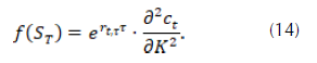
Therefore, the problem of obtaining
is translated to the estimation of c
t
When plotting prices of call options with respect to the strike price for a fixed asset and maturity, we can fit a curve to represent the function, c
t
. We can estimate an adequate function that fits the real values of c
t
by using nonparametric least squares (Yatchew and Härdle, 2006), constrained smoothing splines, Kernel smoothing (Aït-Sahalia and Lo, 1998) or locally polynomial regression (Aït-Sahalia and Duarte, 2003). After c
t
is estimated, the function is differentiated twice to obtain
 . This strategy has some issues, as
must be a density function. In other words, it must be nonnegative, and therefore, c
t
must be monotonically decreasing and convex.
. This strategy has some issues, as
must be a density function. In other words, it must be nonnegative, and therefore, c
t
must be monotonically decreasing and convex.
Although this problem is addressed in the literature by imposing constraints over the estimator, when models are applied to real data, the resultant SPD could be jagged because the second derivative approaches zero for some values of
 or because
 is not smooth since the set of available
values is not continuous (Figure 1). Moreover, whether the estimation of c
t
is parametrical or not, the quality of the estimator with respect to a function’s derivative is much worse than that of the estimator of a function itself (Aït-Sahalia and Duarte, 2003). Indeed, it is even worse for the second derivative. Accordingly, we evaluate methods that avoid differentiation. Ludwig (2015) classified the models as follows: expansion methods, mixture methods, generalized distribution methods and maximum entropy methods. A detailed explanation of his classification is provided in Table 1. Finally, we implement nonparametric mixtures by Yuan (2009) because they allow us to estimate the SPD directly, and they have a high convergence rate.
is not smooth since the set of available
values is not continuous (Figure 1). Moreover, whether the estimation of c
t
is parametrical or not, the quality of the estimator with respect to a function’s derivative is much worse than that of the estimator of a function itself (Aït-Sahalia and Duarte, 2003). Indeed, it is even worse for the second derivative. Accordingly, we evaluate methods that avoid differentiation. Ludwig (2015) classified the models as follows: expansion methods, mixture methods, generalized distribution methods and maximum entropy methods. A detailed explanation of his classification is provided in Table 1. Finally, we implement nonparametric mixtures by Yuan (2009) because they allow us to estimate the SPD directly, and they have a high convergence rate.

Figure 1: From left to right: cost function estimation, first derivative and second derivative of a call option
Source: Authors.
Table 1: Methods of direct SPD estimation.

Nonparametric mixture
With this method, we can create the SDP as the mixture of m lognormal distributions:

where
 is a lognormal density function with mean μ and variance σ 2 evaluated at x and πi is the mixing proportion of the j-th lognormal distribution. It is important to ensure that all the densities in the mixture have the same variance (Yuan, 2009).
Although we cannot compare
 with
with
 , we can compare
 with
with
 This might be confusing as we are not estimating
but
; nevertheless, after estimating
This might be confusing as we are not estimating
but
; nevertheless, after estimating
 , we can use (10) to obtain
 . As
is observable,
must meet the following (Aït-Sahalia and Duarte, 2003):
. As
is observable,
must meet the following (Aït-Sahalia and Duarte, 2003):

where
 is the estimated cost function,
 is the space of possible cost functions,
 is the observed price of the i-th option, and
 is the estimated price of the i-th option. Indeed,
 depends on
 , which is a lognormal distribution; that is,
 relies on
 . The final expression of
 proposed by Yuan (2009) is as follows:

where Φ is the standard cumulative normal distribution and
 .
.
In this way, we create m groups; each group will have
 , and reassigning points between groups (17) changes resulting in different estimators for
 that are input for (16). We iterate minimizing (16) and (15) can be computed.
From the SPD estimation to the portfolio selection problem
After the SPD is estimated, we obtain a probability density function of future prices. However, the parameters of the portfolio selection problem are not based on prices, but on returns. According to Aït-Sahila and Lo (1998), the SPD is related to the distribution of the returns, h(u), as follows:

Proof. If
 is the log return between t and T, then we obtain the following:

Based on this cumulative information, we can find the density as follows:

At the end, our implicit parameters for the mean returns are as follows:

where p is the number of assets in the portfolio. Indeed, we still need to explain the construction of

The historical covariance matrix can be decomposed in a
 diagonal matrix with the standard deviation of the historical returns of the p assets and the
 correlation matrix,
 (DeMiguel et al., 2013):

When our risk measure is the variance, and when we assume that the correlations between assets do not change, the implicit estimator can be described as follows:

where diag
 contains the standard deviation of the SPD (18) for each asset.
If we want to use
 as the risk measure, the estimator is as follows:

where
 contains the VaR of the SPD (18) for each asset, assuming again that correlations are static and using the variance-covariance approach to estimate the VaR of a portfolio (Jorion, 2007). Of course, there are other several ways to estimate the VaR of a portfolio, but this strategy is consistent with our optimization problem.
RESULTS
Data selection
In this study, we evaluated the portfolio performance of S&P 500 stocks. Although present information is easy to obtain, finding historical data is difficult. Moreover, it is crucial to create training and test samples. We obtained the daily bid and ask call and put closing prices for 4,693 symbols in 2016 from the Discount Option Data website. We filtered the data to include only call options from tickers with enough points to conduct the SPD estimation for any day in 2016 and excluded options with bid or ask prices of zero. In addition, we decided that the best estimation of the market price is the average between bid and ask prices. To reduce dispersion, we removed options when the distance between bid and ask was greater than 0,5. This was calculated using (23). Indeed, investors will not sell an asset for any less than what the market will pay for it. In other words, ask is always higher than bid, and the distance is always greater than zero.
Apart from the options database, we used Yahoo Finance as our source of historical security prices from January 2008. Using daily closing prices, we calculated their lognormal returns by time windows; that is, we used the information from when the portfolio was created. For the risk-free rate data, we used the average US Dollar LIBOR interest rate for each month obtained from the Global Rates website.
Algorithm of implementation
The algorithm used to solve the proposed model can be obtained as follows: a date,
t ? T, is selected, where options data for a set of assets, A, is available; we filter options with the expiration, τ days forward; using this data, we estimate the SPD using the nonparametric mixture of lognormal values for each asset; with the estimated SPD in t, we obtain
 .
.
We filter historical information from January 2008 until t for each asset in A. We then create K-folds of historical data to calibrate the model: we remove one fold
 that is kept for testing and we use the rest to estimate the historical parameters,
 with variance as the risk measure. The parameters are then transformed into the same time units before obtaining (7) and (8). As the SPD provides us the estimation of a τ days return, we change each entry of
 , that is, the mean of historical daily returns into that mean multiplied by τ . Accordingly, we decomposed
 like shown in (20), multiply
 and reconstruct
 using (20).
For the problem using the squared VaR risk measure, the mean vector is the same, but we create
 using monthly historical return information (between January 2008 and t) for each asset in A, after which we estimate the
 percentile of the historical information as the VaR of each asset. Then,
 can be expressed using (22).
We can create (7) and (8) by running an elastic net, where X is obtained from (2) with
 and Y is obtained from (3) with

Creating the historical-implicit estimators and running the elastic net requires
 . Therefore, we pick a tuple of the said parameters, create the portfolio, and evaluate the portfolio return using the daily data in
 . We run the model changing the tuple
 for the same fold, after which the process is repeated for each fold. Finally, we average the obtained return for all folds in the selected date together with their VaR values and standard deviations. The selected tuple is the one giving the maximum average objective function among all folds; it is used to create the portfolio weights. With the said weights, we use the portfolio
from
 and there, a new portfolio is created.
We use R to apply the proposed algorithm. Starting in April 2016, we filter the option data of 14 assets with the time to expiration approximal to
 This is because the last month of the option has more realistic information about market expectations.
Firstly, we implement the nonparametric mixture using seven lognormal values. They are initialized with means equally spaced between the natural logarithm of the minimum strike price and the natural logarithm of the maximum strike price available in the set of options of each asset. The standard deviation of all distributions is initialized with 3/4 of their implied volatility (Yuan, 2009). Then, we assign each point to the lognormal distribution that generates best estimation of c. We calculate the mean and standard deviation values of the said groups and use them as the updated parameters of each lognormal. The reassigning process is repeated once for convergence (Yuan, 2009).
After the SPD is estimated, we create the historical-implicit estimators to estimate X and Y. This transformation depends on , a risk aversion coefficient that we set as 3.7 to represent an average investor. We use the glmnet package for the elastic-net model estimation and the Performance Analytics package for the portfolio evaluation.
Model validation
First, we discuss how β and η are chosen by the optimization problem for 2016. In particular, we examine whether the implicit information was considered in the returns or in the risk matrix.
Thereafter, we compare the elastic-net model with historical-implicit estimators and solely historical parameters. As an evaluation tool, we plot the cumulative wealth index of each strategy:

where for each t,

Where
 is the column vector of logarithmic returns of the assets in the portfolio on day
 is the transposed vector of the weights of the investment strategy.
In other words, CW is the resulting amount of money at the end of day t if we invested 1 USD in the portfolio on the first stock day of 2016, and if we reinvested our returns on the portfolio every day until t.
To compare the models, we use the mean absolute deviation and annualized Sharpe ratio (SR) for each strategy; a portfolio with a high SR is desirable. In addition, the information ratio (IR) is calculated to compare how a portfolio with returns, R p , performs over a benchmark portfolio with returns, R b . The IR is the rate between the active premium and the tracking error:

We use the benchmark portfolio for the historical elastic-net model and our portfolio for the historical-implicit elastic-net model using variance or squared VaR. Furthermore, we compare each strategy with the S&P 500 index as a benchmark portfolio. Indeed, we constrain the portfolio weights in our strategies to be nonnegative (no short positions).
Another measure of risk-return relation is the Calmar ratio, which can be used to estimate the relation between the average return and maximum drawdown during a period. A Calmar ratio greater than one is good, greater than three is excellent and above five is more than desirable (Young, 1991). We also provide a plot of the ratio of the cumulative performance of one portfolio with respect to another. In this plot, Portfolio A is better than Portfolio B when the slope is positive; accordingly, we are interested in the evaluation of long periods of overperformance (Peterson et al., 2018).
Data analysis results
Table 2 presents the value of
 for each month and risk measure. A filled cell indicates that implicit information was the only one used in the historical-implicit estimator, whereas an empty cell indicates that the historical-implicit estimator is the same as the historical one. The implicit information of returns and risks are important for the optimization problem, so the portfolios are different from those with historical information alone.
Source: Authors.
Table 2: Weight of implicit information in HI estimators.

From Figure 2, it is evident that both mean-VAR and mean-VaR2 achieve a better performance when using the historical-implicit estimator rather than pure historical estimator. For the mean-VAR portfolio, the cumulative wealth of the historical-implicit estimator is superior during the out-of-sample period, obtaining a final value of 1.28, whereas the historical estimator obtains a final value of 1.24. Indeed, the mean absolute deviation for both portfolios is 0.007, so the historical-implicit estimator has a better return performance for the same level of risk than the historical estimator.

Figure 2: Cumulative wealth index portfolios with historical-implicit vs historical estimators.
In the same way, the historical-implicit model is superior when VaR2 is the risk measure. In this case, the final cumulative wealth value for the historical-implicit portfolio is 2.08 versus 1.71 for the historical one. These portfolios have a mean absolute deviation of 0.012 and a 1-day VaR95% of -0.02, which suggests that, with the same level of risk, the historical-implicit is superior. In this case, the mean-VaR2 has a better result with respect to the mean-VAR problem, but it has a higher level of risk.
When we examine the relative performance plot (Figure 3) to compare the cumulative returns, it is evident that the slope is mainly positive for the mean-VAR and mean-VaR2 problems, proving the advantages of using implicit information. After recognizing historical-implicit superiority, we compare this strategy with the passive index strategy. Figure 4 presents the historical-implicit estimators; the resultant portfolios have a superior out-of-sample performance compared with the passive index strategy.

Figure 3: Relative performance plot for portfolios with historical-implicit estimator and portfolios with historical estimators as a benchmark

Figure 4: Relative performance plot for portfolios using historical-implicit estimators with S&P 500 as a benchmark.
Table 3 presents the portfolio performance indicators, where MVH denotes the mean-VAR problem using historical estimators; MVHI, the mean-VAR problem using historical-implicit estimators; M@H, the mean-VaR2 problem with historical estimators; and M@HI, the mean-VaR2 problem with historical-implicit estimators. The annualized SR was calculated using a 0,4% risk-free rate (average rate of 2016); it gives a good result for every portfolio. In both cases, the portfolios that use the historical-implicit estimators are better. This is the same for the Calmar ratio, which is also better for the historical-implicit portfolios. A Calmar ratio larger than three constitutes an excellent performance for all our strategies. Indeed, the M@HI strategy outperforms the others in terms of the SR and the Calmar ratio.
Table 3. Portfolio performance indicators.

Source: Authors.
Table 4 presents the IR values, from which it is evident that the IR of the MVHI is 0.44. Because this value is larger than 0.4, the MVHI can generate better returns for longer periods of time than the MVH. Moreover, it is significantly better than the passive index strategy, as it has a value of 1.83, whereas a high-level investor can only achieve an IR of 1.5 in the S&P 500. For the M@HI, we can conclude that it outperforms the M@H with respect to the risk-return relationship, as the IR is larger than five. In addition, this portfolio has also an excellent behavior when the S&P 500 index is used as a benchmark.
Table 4. IR.

Source: Authors.
Conclusions
Multiple portfolio selection methodologies have been developed since Markowitz. However, during the last decade there have been many improvements to adjust the performance of the portfolio using real data as the input information. In this paper, we constructed the SPD and estimated the return density function for each asset. We applied our historical-implicit estimators for the returns and risk measure. In addition, we constrained the L1 and L2 norms of the vector of weights to reduce the risk of all estimations.
The results suggest that the model has a good out-of-sample performance. It is superior to models with pure historical estimations; moreover, it is also a good portfolio in terms of cumulative returns and risk return relation measured by the SR, IR and Calmar ratio.
Acknowledgements
Acknowledgements
This research did not receive any specific grant from funding agencies in the public, commercial, or not-for-profit sectors.
References
License
Copyright (c) 2020 Carlos Felipe Valencia-Arboleda, Diego Hernan Segura-Acosta

This work is licensed under a Creative Commons Attribution-NonCommercial-ShareAlike 4.0 International License.
When submitting their article to the Scientific Journal, the author(s) certifies that their manuscript has not been, nor will it be, presented or published in any other scientific journal.
Within the editorial policies established for the Scientific Journal, costs are not established at any stage of the editorial process, the submission of articles, the editing, publication and subsequent downloading of the contents is free of charge, since the journal is a non-profit academic publication. profit.

