DOI:
https://doi.org/10.14483/23448393.18538Published:
2022-04-25Issue:
Vol. 27 No. 2 (2022): May-AugustSection:
Sección Especial: Mejores artículos extendidos - WEA 2021Testing the Causes of a Levee Failure Using Bayesian Networks
Evaluación de las causas de falla de un dique usando redes bayesianas
Keywords:
forensic geotechnical engineering, Bayesian Networks, levee failure (en).Keywords:
ingeniería geotécnica forense, redes bayesianas, falla de diques (es).Downloads
References
F. Taroni, A. Biedermann, P. Garbolino, and C. G. G. Aitken, “A general approach to Bayesian networks for the interpretation of evidence,” Forensic Sci. Int., vol. 139, no. 1, pp. 5-16, 2004. https://doi.org/10.1016/j.forsciint.2003.08.004 DOI: https://doi.org/10.1016/j.forsciint.2003.08.004
M. Neil, N. Fenton, D. Lagnado, and R. D. Gill, “Modelling competing legal arguments using Bayesian model comparison and averaging,” Artif. Intell. Law, vol. 27, no. 4, pp. 403-430, 2019. https://doi.org/10.1007/s10506-019-09250-3 DOI: https://doi.org/10.1007/s10506-019-09250-3
P. Garbolino and F. Taroni, “Evaluation of scientific evidence using Bayesian networks,” Forensic Sci. Int., vol. 125, no. 2-3, pp. 149-155, 2002. https://doi.org/10.1016/S0379-0738(01)00642-9 DOI: https://doi.org/10.1016/S0379-0738(01)00642-9
A. Biedermann and F. Taroni, “Bayesian networks for evaluating forensic DNA profiling evidence: A review and guide to literature,” Forensic Sci. Int. Genet., vol. 6, no. 2, pp. 147-157, 2012. https://doi.org/10.1016/j.fsigen.2011.06.009 DOI: https://doi.org/10.1016/j.fsigen.2011.06.009
M. Kwan, R. Overill, K.-P. Chow, H. Tse, F. Law, and P. Lai, “Sensitivity analysis of Bayesian networks used in forensic investigations,” IFIP Adv. Inf. Commun. Technol., vol. 361, pp. 231-243, 2011. https://doi.org/10.1007/978-3-642-24212-0_18 DOI: https://doi.org/10.1007/978-3-642-24212-0_18
G. A. Davis, “Bayesian reconstruction of traffic accidents,” Law. Probab. Risk, vol. 2, no. 2, pp. 69-89, 2003. https://doi.org/10.1093/lpr/2.2.69 DOI: https://doi.org/10.1093/lpr/2.2.69
M. Holický, V. Návarová, R. Gottfried, M. Kronika, J. Marková, and K. J. Miroslav Sýkora, Basics for assessment of existing structures, Prague, Czech Rep.: Kolkner Institute, Czech Technical University in Prague, 2013.
A. Biedermann, F. Taroni, O. Delemont, C. Semadeni, and A. C. Davison, “The evaluation of evidence in the forensic investigation of fire incidents (Part I): An approach using Bayesian networks,” Forensic Sci. Int., vol. 147, no. 1, pp. 49-57, 2005. https://doi.org/10.1016/j.forsciint.2004.04.014 DOI: https://doi.org/10.1016/j.forsciint.2004.04.014
A. Biedermann, F. Taroni, O. Delemont, C. Semadeni, and A. C. Davison, “The evaluation of evidence in the forensic investigation of fire incidents. Part II. Practical examples of the use of Bayesian networks,” Forensic Sci. Int., vol. 147, no. 1, pp. 59-69, 2005. https://doi.org/10.1016/j.forsciint.2004.04.015 DOI: https://doi.org/10.1016/j.forsciint.2004.04.015
Y. Xu and L. Zhang, “Diagnosis of Geotechnical Failure Causes Using Bayesian Networks,” in Forensic Geotechnical Engineering, V. V. S. Rao and G. L. Sivakumar Babu, Eds. New Delhi: Springer India, 2016, pp. 103-112. DOI: https://doi.org/10.1007/978-81-322-2377-1_6
P. Grubert, “Saaledeich bei Breitenhagen Geotechnische Untersuchungen der Bruchstelle Empfehlungen zur Sanierung,” Magdeburg, Ger.: Gesellschaft für Grundbau und Umwelttechnik mbH, 2013.
J. J. Kool, W. Kanning, T. Heyer, C. Jommi, and S. N. Jonkman, “Forensic analysis of levee failures: the Breitenhagen case,” Int. J. Geoengin. Case Hist., vol. 5, no. 2, pp. 70-92, 2019. https://doi.org/10.4417/IJGCH-05-02-02
J. J. Kool, W. Kanning, C. Jommi, and S. N. Jonkman, “A Bayesian hindcasting method of levee failures applied to the Breitenhagen slope failure,” Georisk Assess. Man. Risk Eng. Sys. Geohazards, vol. 15, no. 4, pp. 299-316, 2020. https://doi.org/10.1080/17499518.2020.1815213 DOI: https://doi.org/10.1080/17499518.2020.1815213
V. V. S. Rao and G. L. S. Babu, Forensic Geotechnical Engineering, India: Springer India, 2016.
G. L. S. Babu, “Briefing: Forensic geotechnical engineering,” in Proceedings of the Institution of Civil Engineers - Forensic Engineering, vol. 164, no., 2016, pp. 123-126. http://dx.doi.org/10.1680/jfoen.16.00025 DOI: https://doi.org/10.1680/jfoen.16.00025
ASCE, Guidelines for Failure Investigation, Reston, VA, USA: American Society of Civil Engineers (ASCE), 2018.
S. P. Brady, “Role of the forensic process in investigating structural failure,” J. Perform. Constr. Facil., vol. 26, no. 1, pp. 2-6, 2012. https://doi.org/10.1061/(ASCE)CF.1943-5509.0000274 DOI: https://doi.org/10.1061/(ASCE)CF.1943-5509.0000274
K. L. Carper, Ed., Forensic engineering, Boca Ratón, FL, USA: CRC Press, 2000.
J. B. Kardon, Guidelines for forensic engineering practice, vol. 7, no. 2, VA, USA: American Society of Civil Engineers (ASCE), 2003.
R. Noon, Scientific method: applications in failure investigation and forensic science. Boca Raton, FL, USA: CRC Press, 2009. DOI: https://doi.org/10.1201/9781420092813
R. T. Ratay, Ed., Forensic structural engineering handbook, New York, NY, USA: McGraw-Hill, 2000.
K. Terwel, M. Schuurman, and A. Loeve, “Improving reliability in forensic engineering: The Delft approach,” Proc. Inst. Civ. Eng. Forensic Eng., vol. 171, no. 3, pp. 99-106, 2018. https://doi.org/10.1680/jfoen.18.00006 DOI: https://doi.org/10.1680/jfoen.18.00006
H. G. Poulos, “A Framework for Forensic Foundation Engineering,” in Forensic Geotechnical Engineering, V. V. S. Rao and G. L. Sivakumar Babu, Eds. New Delhi, India: Springer India, 2016, pp. 1-15. DOI: https://doi.org/10.1007/978-81-322-2377-1_1
J. Spross, F. Johansson, L. K. T. Uotinen, and J. Y. Rafi, “Using observational method to manage safety aspects of remedial grouting of concrete dam foundations,” Geotech. Geol. Eng., vol. 34, no. 5, pp. 1613-1630, 2016. https://doi.org/10.1007/s10706-016-0069-8 DOI: https://doi.org/10.1007/s10706-016-0069-8
G. R. Bell, “Engineering investigation of structural failures,” in Forensic Structural Engineering Handbook, R. T. Ratay, Ed. New York, NY, USA: McGraw-Hill, pp. 211-243, 2000.
R. N. Hwang, “Back analyses in forensic geotechnical engineering,” in Forensic Geotechnical Engineering, V. V. S. Rao and G. L. Sivakumar Babu, Eds. New Delhi, India: Springer India, 2016, pp. 131-143. DOI: https://doi.org/10.1007/978-81-322-2377-1_9
V. V. S. Rao, “Guidelines for forensic investigation of geotechnical failures,” in Forensic Geotechnical Engineering, V. V. S. Rao and G. L. Sivakumar Babu, Eds. New Delhi, India: Springer India, 2016, pp. 39-44. DOI: https://doi.org/10.1007/978-81-322-2377-1_3
M. Holický, J. Marková, and M. Sýkora, “Forensic assessment of a bridge downfall using Bayesian networks,” Eng. Fail. Anal., vol. 30, pp. 1-9, 2013. https://doi.org/10.1016/j.engfailanal.2012.12.014 DOI: https://doi.org/10.1016/j.engfailanal.2012.12.014
K. K. Phoon, G. L. Sivakumar Babu, and M. Uzielli, “Role of reliability in forensic geotechnical engineering,” in Forensic Geotechnical Engineering, V. V. S. Rao and G. L. Sivakumar Babu, Eds. New Delhi, India: Springer India, 2016, pp. 467-491. DOI: https://doi.org/10.1007/978-81-322-2377-1_31
F. V. Jensen and T. D. Nielsen, Bayesian networks and decision graphs. New York, NY, USA: Springer, 2007. DOI: https://doi.org/10.1007/978-0-387-68282-2
D. Koller and N. Friedman, Probabilistic graphical models: principles and techniques. London, England: The MIT Press, 2009.
M. Kwan, K.-P. Chow, L. Frank, and P. Lai, “Reasoning about evidence using Bayesian networks,” in Advances in Digital Forensics IV. DigitalForensics 2008. IFIP — The International Federation for Information Processing, vol. 285, I. Ray and S. Shenoi, Eds., Boston, MA, USA, Springer, 2008, pp. 275-289. https://doi.org/10.1007/978-0-387-84927-0_22 DOI: https://doi.org/10.1007/978-0-387-84927-0_22
N. Fenton and M. D. Neil, Risk assessment and decision analysis with bayesian networks, Boca Raton, FL, USA: CRC Press, 2019. DOI: https://doi.org/10.1201/b21982
L. M. de Campos, J. A. Gámez, and S. Moral, “Simplifying explanations in Bayesian belief networks,” in International Journal of Uncertainty, Puzziness and Knowledge-Based Systems, vol. 9, no. 4, pp. 461-489, 2001. https://doi:10.1142/s0218488501000892 DOI: https://doi.org/10.1142/S0218488501000892
J. Pearl, Probabilistic Reasoning in Intelligent Systems: Networks of Plausible Inference, San Francisco, CA, USA: Morgan Kaufmann Publishers Inc., 1988.
B. Seroussi and J. L. Golmard, “An algorithm directly finding the K most probable configurations in Bayesian networks,” Int. J. Approx. Reason., vol. 11, no. 3, pp. 205-233, 1994. https://doi.org/10.1016/0888-613X(94)90031-0 DOI: https://doi.org/10.1016/0888-613X(94)90031-0
U. B. Kjærulff, A. L. Madsen, Bayesian networks and influence diagrams: A guide to construction and analysis, New York, NY, USA: Springer, 2013. DOI: https://doi.org/10.1007/978-1-4614-5104-4
V. K. D. Mohan, P. J. Vardon, M. A. Hicks, and P. H. A. J. M. van Gelder, “Uncertainty tracking and geotechnical reliability updating using Bayesian networks Varenya,” in Proceedings ofthe 7th InternationalSymposiumonGeotechnical SafetyandRisk(ISGSR), 2019, no. December, pp. 978-981. https://doi.org/10.3850/978-981-11-2725-0 DOI: https://doi.org/10.3850/978-981-11-2725-0-IS3-5-cd
R. van der Meij, “D-Stability. Slope stability software for soft soil engineering,” Deltares, Sep. 2020. https://www. https://download.deltares.nl/en/download/d-stability/(accesed Nov. 30, 2020).
How to Cite
APA
ACM
ACS
ABNT
Chicago
Harvard
IEEE
MLA
Turabian
Vancouver
Download Citation
Recibido: 30 de diciembre de 2021; Revisión recibida: 18 de noviembre de 2021; Aceptado: 9 de febrero de 2022
Abstract
Context:
Forensic geotechnical engineering aims to determine the most likely causes leading to geotechnical failures. Standard practice tests a set of credible hypotheses against the collected evidence using backward analysis and complex but deterministic geotechnical models. Geotechnical models involving uncertainty are not usually employed to analyze the causes of failure, even though soil parameters are uncertain, and evidence is often incomplete.
Method:
This paper introduces a probabilistic model approach based on Bayesian Networks to test hypotheses in light of collected evidence. Bayesian networks simulate patterns of human reasoning under uncertainty through a bidirectional inference process known as “explaining away.” In this study, Bayesian Networks are used to test several credible hypotheses about the causes of levee failures. Probability queries and the K-Most Probable Explanation algorithm (K-MPE) are used to assess the hypotheses.
Results:
This approach was applied to the analysis of a well-known levee failure in Breitenhagen, Germany, where previous forensic studies found a multiplicity of competing explanations for the causes of failure. The approach allows concluding that the failure was most likely caused by a combination of high phreatic levels, a conductive layer, and weak soils, thus allowing to discard a significant number of competing explanations.
Conclusions:
The proposed approach is expected to improve the accuracy and transparency of conclusions about the causes of failure in levee structures.
Keywords:
forensic geotechnical engineering, Bayesian Networks, levee failure.Resumen
Contexto:
La ingeniería geotécnica forense tiene como objetivo determinar las causas más probables que conducen a fallas de tipo geotécnico. La práctica habitual pone a prueba un conjunto de hipótesis a la luz de la evidencia, utilizando análisis retrospectivos y modelos geotécnicos complejos pero deterministas. Los modelos geotécnicos que involucran incertidumbre no suelen emplearse para analizar las causas de falla, a pesar de que los parámetros del suelo son inciertos y la evidencia suele ser incompleta.
Método:
Este artículo presenta un enfoque de modelo probabilístico basado en redes bayesianas para evaluar hipótesis con base en la evidencia recolectada. Las redes bayesianas simulan patrones de razonamiento humano bajo incertidumbre a través de un proceso de inferencia bidireccional conocido como explaining away [explicación]. En este estudio, las redes bayesianas se utilizan para probar hipótesis creíbles sobre las causas de falla de un dique. Para evaluar las hipótesis se utilizan consultas de probabilidad y el algoritmo de explicación más probable (K-MPE).
Resultados:
El enfoque se empleó en el análisis de un dique en Breitenhagen, Alemania, donde varios estudios forenses anteriores encontraron multiplicidad de explicaciones contrapuestas acerca de las causas de falla. El enfoque permite concluir que la causa más probable de falla fue una combinación de altos niveles freáticos, una capa de suelo de alta permeabilidad y suelos de baja resistencia, lo que permitió descartar un número significativo de explicaciones contrapuestas.
Conclusiones:
Se espera que el enfoque probabilístico propuesto mejore la precisión y la transparencia de las conclusiones sobre las causas de falla en estructuras tipo dique.
Palabras clave:
ingeniería geotécnica forense, redes bayesianas, falla de diques..Introduction
Drawing conclusions about the causes of geotechnical failures can be strongly affected by parameters and model uncertainties. Therefore, conclusions derived from forensic assessments often seem to be arbitrary and controversial. Although forensic analyses follow a rigorous process, the lack of a probability-based framework can lead to costly and inefficient engineering solutions, as well as to the wrong legal decisions.
Graphical probabilistic methods such as Bayesian Networks (BNs) can improve the practice of forensic geotechnical engineering. Their ability to model competing hypotheses about the causes of failure makes them a suitable tool for forensic assessments. BNs have been mainly used in medicine, legal, and forensic science, mostly to support decisions in circumstances where uncertainty or imprecision prevails 1)(5. Forensic engineering has partially used BNs for drawing reasonable conclusions about the causes of failures. Several studies, such as those presented in 6)-(9, demonstrate their applicability. Despite the benefits of BNs in forensic engineering, they have not been widely adopted in forensic geotechnical studies 10.
This paper presents a Bayesian Network approach to support decisions in forensic geotechnical assessments. The approach relies on the generic forensic engineering process for failure assessment but incorporates a probabilistic framework to consider parameters and model uncertainties. The Breitenhagen levee failure that occurred in Germany in 2013 is used to validate the proposed BN approach. Data, studies, and some assumptions associated with the Breitenhagen levee failure, which are presented in 11, 12, and 13, are used as a starting point for this study.
The results show that the proposed BN approach can support the forensic geotechnical process. Moreover, the interpretability and traceability of BNs ensure a rational decision based on a probabilistic framework. Therefore, legal decisions and engineering solutions can be supported by more objective conclusions.
Forensic geotechnical engineering
Forensic geotechnical engineering deals with investigating and communicating the causes of failures attributed to geological/geotechnical aspects 14, 15. It involves the analysis of cause-effect relationships using the scientific method and some complementary techniques. Most forensic engineering methodologies focus on structural failures 16. However, very few procedures and guidelines have been adapted to fulfil forensic geotechnical requirements. Among them, there is a methodology for levee failures 12, a conceptual framework proposed in 23, and a modified version of the observational method 24.
From a broader perspective, this process includes four stages 16, 17: (1) collecting evidence, (2) developing failure hypotheses, (3) testing hypotheses against evidence, and (4) finding the most likely cause of failure. In the first stage, forensic engineers collect all available information to understand the circumstances that led to the failure. Sources of information may include field observations and investigation, traditional and drone photography, working drawings, contract documents, eyewitness interviews, and construction records 16.
The second stage aims to develop credible hypotheses of failure based on the collected evidence. Brady 17 and Bell 25 suggest that conventional design methods used in engineering practices are not suitable for developing credible hypotheses. These methods apply synthesis techniques based on forwarding reasoning. Synthesis could lead to wrong conclusions about the causes of failure because the collected evidence is forced to match biased hypotheses. 20 recommends deductive analysis to investigate the causes of failures, where the collected evidence guides the development of credible hypotheses.
In the third stage, hypotheses about the causes of failure are tested against the collected evidence. Back analysis has been commonly used to accept or reject hypotheses. However, selecting analytical tools and interpreting results from back analysis requires experienced engineers 26, mainly when the failure is represented by complex soil constitutive models and demanding analytical tools.
The fourth stage is the goal of any forensic assessment. A credible cause of failure is reached when all alternative hypotheses are eliminated and only one (or some) match the evidence. Selecting the most likely cause (or causes) of failure is quite a challenging task. Occasionally, the selected cause of failure seems arbitrary or subjective due to large uncertainties in both parameters and models 12, 25 and 20 suggest using the scientific method to overcome subjectivity. The scientific method tests hypotheses against the collected evidence in order to approve or disapprove its validity. In other words, the method reexamines the collected evidence to determine if a hypothesis can explain it.
In forensic geotechnical engineering, 23 and 27 propose some guidelines based on the scientific method. 20 goes further and argues that reliable scientific interpretations about causes of failure should come from statistic and probabilistic analysis. To date, very few forensic engineering assessments use probabilistic tools 13, 28. Furthermore, 29 recognize the scarcity of previous literature about this topic.
Bayesian Networks
This section introduces some important concepts regarding Bayesian Networks (BNs). Several standard textbooks, such as 30 and 31, are recommended for an extended introduction. A BN is a probabilistic model that combines probability and graph theories 32. BNs are used for inference and reasoning under uncertainty due to their ability to simulate human reasoning processes 33. Forward and backward inference is recognized as a crucial characteristic in BNs. These attributes, along with a rigorous probabilistic background, have led BNs to successful applications 1, 2, 5, 6. In the technical literature, BNs are also known as Bayesian expert systems, probabilistic graphic networks, belief networks, or Bayes nets.
Basic definitions
A problem involving reasoning under uncertainty and decision-making can be represented through a causal graph G (see Fig. 1). G is a structure consisting of nodes and edges1. Nodes represent events or variables, and edges embody causal relationships between nodes 31. A pair of nodes Xj and Xj, belonging to a set of nodes X = {X1,..., Xn}, can be connected by a directed edge Xi ? Xj. When the edges in G do not form a cycle, G is known as a directed acyclic graph (DAG). Nodes encode random variables, propositions, or sample spaces. A node can have any number of states in a discrete set or in a continuous set. For example, node Xi in Fig. 1 has two states Xj = {Xi 0,Xj 1}, whereas the sample space of node Xj is described by a Gaussian distribution Xj ~ N(μXj ; σ Xj ).
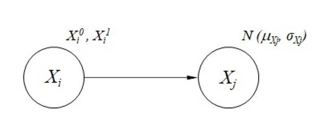
Figure 1: A simple causal graph G
Causal relationships between nodes X are graphically represented by edges E. In the context of BNs, causality denotes dependencies between variables or the direct influence of node Xi on node Xj. Usually, this influence is not entirely deterministic. Therefore, E expresses the probabilistic influence of Xj on Xj. For discrete variables, the influence is represented by a conditional probability table (CPT). In the case of continuous variables, conditional probability distributions (CPD) are employed. A CPT specifies a probability distribution over the states of Xj given each possible state of Xi. In more general terms, a CPT encodes P(Xj|pa(Xj)), where pa(Xi) represents the set of nodes in X with edges pointing to Xi. The term pa(Xi) is read as parents of Xi.
A causal graph is defined as a Bayesian Network when all the following conditions are met 30:
-
Each node has a finite set of mutually exclusive states.
-
The edges do not form a cycle between nodes (i.e., it is a DAG).
-
The strength of the causal relationship between variables is expressed by conditional probabilities tables or distributions (CPTs or CPDs).
Structure of a Bayesian Network
The structure of a BN refers to the type of relationships (connections) between nodes. There are three basic connections in a BN: serial, converging, and diverging. Each type of connection determines which nodes are updated when some evidence is entered in the BN.
A serial connection between three nodes is shown in Fig. 2a. In this structure, node A influences B, which in turn influences C. If the state of A is known (i.e., A is instantiated), it will influence the state of C through node B. Similarly, if the state of C is known, the state of A will change through B. On the contrary, if the state of node B is known, the flow of information between A and C is blocked. In this case, A and C are d-separated given B.
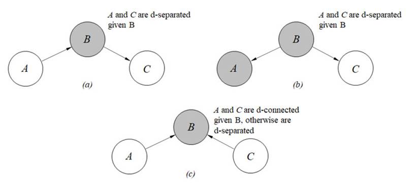
Figure 2: Basic connections in BNs: (a) serial connection, (b) diverging connection, (c) converging connection. Grey nodes indicate instantiation
Fig. 2b presents a diverging connection between three nodes. If some evidence is included in B, information is transmitted to A and C. However, any additional evidence included in A when B is instantiated will not be transferred to C. In this case, A and C are d-separated given B, or A and C are conditionally independent given B.
In a converging connection (Fig. 2c), any evidence entered in A and C will change the state of node B. Likewise, any evidence included in B will change the state of A and C. Hence, A and C can transmit information between them when B is instantiated. In other words, A and C are d-connected given B. In any other case, A and C are d-separated.
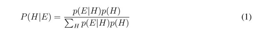
The power of BNs resides on combining Bayes’s rule and the chain rule. These characteristics give BNs the ability for decision-making and abductive reasoning. Bayes’s rule states that prior belief about a hypothesis can be modified if some evidence is available. Let us say that H represents a hypothesis and E some evidence related to H. The updated belief about H given E can be calculated through Bayes’s rule (Eq. 1). In Eq. 1, P(H|E) represents the posterior (updated) probability of H given E, P(E|H) the likelihood of the evidence given the hypothesis H, and P(H) the prior probability of H. The term in the denominator is the marginal likelihood, which normalizes the posterior probability.
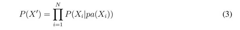
The chain rule reflects the properties of a BN. Let X' = {A, B, C, D, E} be the universe of variables that describe a problem. If GBN defines a Bayesian network over X' (Fig. 3), then Eq. (2) represents the conditional probability of GBN, where A and B are parent nodes and C, D, and E are children nodes. Eq. (2) can be rewritten in the compact form of Eq. (3). Although a GBN is sufficient for updating probabilities, BNs with many nodes have a high computational cost. Some efficient algorithms such as junction three and stochastic simulation considerably reduce this cost.
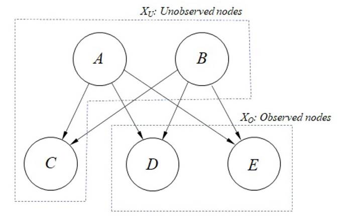
Figure 3: Example of a BN with five nodes: two parents and three children. Dash lines indicate sets of observed and unobserved nodes.

Abductive reasoning in Bayesian Networks
BNs play a significant role in the field of abductive reasoning methods. Abduction refers to generating plausible explanations (hypotheses) for a set of observations (evidence) related to a phenomenon. Fig. 4 presents the abductive process described in 34 adapted to the geotechnical context. Based on the collected evidence and observed behavior, several credible hypotheses are generated. These hypotheses constitute a set of possible explanations for a geotechnical failure (i.e., causes of failure). A BN, along with a metric-based criterion, is used to select the most probable hypothesis (i.e., the best explanation).
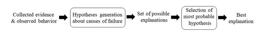
Figure 4: Abductive process 34 adapted to the geotechnical context.
Let xo be a set of collected evidence for the observed nodes XO in a BN (Fig. 3). An explanation is an arrangement of states for the unobserved nodes XU = xU that is consistent with xo. Abductive reasoning aims to find the best explanation (Most Probable Explanation, MPE) among a set of possible explanations 35. Eq. (4) defines the MPE in which x* U is a single arrangement of states for Xu. Although the MPE is a useful metric, abductive reasoning is also interested in the KMost Probable Explanations (K-MPE) 36. The K-MPE identifies and organizes the most probable states of Xu according to their joint probabilities.

Bayesian Network approach for forensic assessment of a levee failure
Assessing evidence and evaluating competing hypotheses are regarded as challenging tasks 15, 18. Abductive and probabilistic reasoning can support these tasks through the rigorous mathematical frame-work of BNs. The five-step approach proposed in this paper is described in the following subsections. In general, the approach defines a set of competing hypotheses about the causes of a levee failure and builds a BN to test them. The collected evidence is included in the BN to assess the hypotheses via an abductive process. The approach identifies the most probable causes of failure (explanations) using the K-MPE metric over the set of credible hypotheses.
The five-step approach
The first step consists of identifying credible hypotheses about the causes of failure. In geotechnical engineering, common failure hypotheses are related to pore water pressures, loading magnitudes, and subsoil conditions 13. Each credible hypothesis is translated into the BN through a node. Subsequently, several states are assigned to each node according to its characteristics.
The second step defines evidence nodes to the observed or behavioral variables. These nodes can include, among others, stability condition, deformation magnitude, water level elevation, runout distance, and slip geometry. In some cases, mediating variables could be required to connect hypotheses and evidence nodes. For example, the Factor of Safety (FoS) can be defined as a mediating variable to link a hypothesis node related to the soil strength and an evidence node associated with the stability condition.
Given the set of hypotheses and observed nodes, the next step identifies causal relationships between nodes. Causality is easily identifiable when a physical model of the phenomenon is available. Otherwise, the BN structure can be supported on semantic and syntax substructures known as idioms 37. It is easily identifiable by expressions such as ‘attributable to, due to, as a consequence of, impact, caused by, resulting in’, among others.
Once the causal graph has been defined (i.e., nodes and edges), the fourth step aims to elicit the conditional probability tables (CPT). This quantitative information can be obtained from mathematical models (e.g., computer simulations) or databases. Expert knowledge can also be used to determine the CPD values. However, analyses with multiple nodes could limit the use of expert knowledge.
The final step involves entering the collected evidence into the BN, updating the nodes, and evaluating the competing hypotheses. In this step, the BN is used to answer questions in the form of conditional probability queries, in other words, to find the probabilities of unobserved nodes given specific states in observed nodes 38. The K-MPE is a particular type of query that aims to identify the K most likely states of the nodes given some evidence. Its results can be used to draw conclusions about the causes of failure. In this study, hypotheses describing the causes of failure from a forensic perspective are statistically compared by evaluating their likelihoods.
Application example: the Breitenhagen levee failure
The proposed five-step BN approach was applied to the Breitenhagen levee failure. 12 presented a comprehensive forensic study of this case based on a sensitivity analysis. The failure scenarios and geotechnical models presented in 12 are used to validate the proposed BN approach.
General description
The Breitenhagen levee failure occurred in June 2013 during the Sale River floods in SaxonyAnhalt, Germany. According to 11, the failure was a slope instability due to sustained high water levels in both the Elbe and Saale rivers. The levee at the failure location was 3,5 m high with a 3,0 m wide crest. The slope at the waterside was 1V:3,1H, whereas the slope at the landside was 1V:2,1H.
Fig. 5 presents a cross-section of the levee and a simplified stratigraphy inferred from borings reported in 11. The levee consists mainly of two soil layers. The upper soil is a homogeneous cohesive material, underlain by a sandy soil at about 5,5 m below the levee's crest.

Figure 5: The Breitenhagen levee at the failure location, cross-section, and simplified stratigraphy. NHN (Normalhohennull) corresponds to the vertical datum used in Germany
Some authors conducted forensic assessments to determine the causes of the Breitenhagen levee failure. For example, 11 concluded that the most likely cause of failure was the existence of a conductive layer inside the levee. 12 used a series of photographs taken at the moment of failure to infer a circular slip surface. These authors also identified a pond by the waterside, indicating a possible connection between the aquifer (sand layer) and the landside. A later study, 13, determined that the failure was likely caused by locally weak soils and high water pore pressures in the aquifer. The proposed BN approach is applied and explained in detail in the following sections.
Step 1. Identification of hypothesis nodes
Hypotheses about possible causes of failure are defined using the evidence collected from previous studies 11, 12. Two sets of hypotheses are identified. The first set includes three hypotheses related to the following pore pressure conditions (Fig. 6):
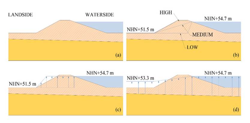
Figure 6: Levee models for hypotheses related to pore pressure conditions: (a) basic model, (b) phreatic level elevations, (c) existence of a conductive layer, (d) existence of high pore pressures inside the levee due to a pond connection
Table I: Definition of hypothesis nodes and their corresponding states
Node
Definition
Distribution
States
PL
Phreatic line elevation
Discrete uniform
High, Medium, Low
CL
High pore pressures inside the levee due to a conductive layer
Discrete uniform
Yes, No
PC
High pore pressures inside the levee due to a pond connection (PC) to the aquifer
Discrete uniform
Yes, No
c’
Effective cohesion intercept (Mohr-Coulomb constitutive model) in kPa
Discrete uniform
[0, 1, 2, …, 15]
(‘
Angle of shear resistance in degrees
Discrete uniform
[15, 16, …, 33, 34]
S
Normally consolidated stress ratio
Discrete uniform
[0.23, 0.25, 0.27, …, 0.49]
m
Strength increase exponent
Discrete uniform
[0.50, 0.54, 0.58, …, 0.98]
POP
Pre-Overburden Pressure
Discrete uniform
[0, 10, 20, …, 150]
-
phreatic level elevation,
-
existence of a conductive layer, and
-
existence of high pore pressures inside the levee due to a pond connection.
The second set consists of hypotheses associated with the parameters of two soil models: MohrCoulomb for drained conditions and SHANSEP for undrained behavior. The Mohr-Coulomb model includes the parameters ^'(effective angle of shear resistance) and c’ (effective cohesion intercept). The SHANSEP model contains the parameters S (normally consolidated stress ratio), m (strength increase exponent), and POP (pre-overburden pressure).
A unique node is assigned to each pore pressure condition and each soil parameter. For the sake of simplicity, discrete values are used to describe the set of possible states of each node.
Step 2. Definition of evidence nodes
Two evidence nodes are defined to account for observed or behavioral variables. The first node corresponds to the levee’s stability condition. This node includes two states: stable and unstable. The stability condition is usually evident and only requires visual inspection. However, some cases require the evaluation of experienced engineers. For the Breitenhagen failure, the unstable condition was inferred from photographs taken during the event 11. The consequences of the failure (e.g., floods) may also be used to define the levee’s stability condition.
The second evidence node refers to the slip surface geometry. Identifying and measuring slip surfaces is a challenging task. Slip surfaces usually disappear after failure or cannot be fully observed. In some cases, the start and end locations of slip surfaces are identifiable. For the Breitenhagen failure, six start and six end locations were defined. Each location represents a possible interval within which start and end points can be observed.
Fig. 7 presents an example of two entry and exit intervals, as well as two potential circular slip surfaces. A total of 36 start-end point combinations are defined. Table II presents the evidence nodes used in the analysis and their corresponding states.
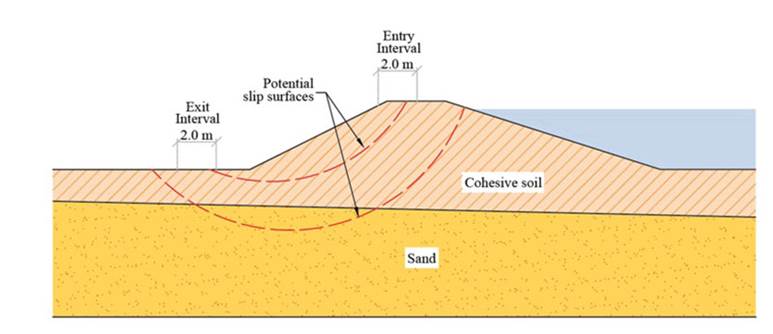
Figure 7: Example of potential slip surfaces with entry and exit intervals. Start and end points of slip failures can be observed within these intervals
Table II: Definition of evidence nodes and their corresponding states
Node
Definition
Distribution
States
SC
Stability condition
Discrete
Stable, Unstable
SG
Slip surface geometry
Discrete
36 geometries: SG1 to SG36 (Locations defined based on levee geometry and circular failure mechanisms)
Step 3. Causal connections
The causal relationships between hypothesis nodes and evidence nodes are defined using mathematical models and semantic substructures. Bishop’s limit equilibrium equations are used to infer causal connections between nodes representing soil parameters and evidence nodes. On the other hand, causal connections between hypothesis nodes related to pore pressure conditions and evidence nodes are deduced from semantic substructures. For instance, (12, p. 70) describes the causes of levee failure in the following terms: “the levee breach is likely caused by unexpected high pore pressures (...) and unexpected saturation of the levee”. (11, p. 35) (translated from German) describes the causes of failure as follows: “the primary cause of damage is a combination of several partial causes such as (... ) horizontal water seepage due to a root zone on the waterside”. The causal graphs for both Mohr-Coulomb and SHANSEP models are presented in Fig. 8.
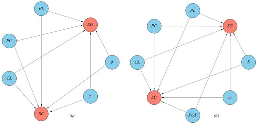
Figure 8: Causal graphs for the Breitenhagen failure analysis: (a) Mohr-Coulomb (drained) constitutive model, (b) SHANSEP (undrained) soil model
Step 4. Elicitation of conditional probability distributions
The elicitation of conditional probability tables (CPTs) consists of two phases. The first phase includes the definition of prior probabilities for hypothesis nodes. In the case of Breitenhagen failure, no prior knowledge about the causes of failure is available. Therefore, states for each hypothesis node are equally probable and described by discrete uniform distributions.
The second phase involves eliciting the CPTs for evidence nodes. A numerical experiment consisting of 200.000 Monte Carlo simulations is used to infer these CPTs. In the experiment, a random sequence of states is generated based on the prior probabilities of hypothesis nodes. Each sample from the sequence is tested via a slope stability analysis using D-Stability 39 and a Python script. Bishop’s equations are implemented in the slope stability calculations.
The set of results from the calculations (i.e., stability condition and slope geometry) are used to elicit the CPTs of evidence nodes and described by discrete distributions using the states presented in Table II.
Fig. 9 and Fig. 10 depict the BNs for the Breitenhagen failure along with their prior distributions (i.e., no evidence) for both hypotheses and evidence nodes.

Figure 9: BN for the drained constitutive model (Mohr-Coulomb) before observing any evidence
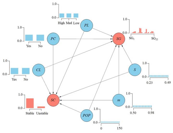
Figure 10: BN for the SHANSEP soil model before observing any evidence
Step 5. Entering evidence and evaluating competing hypotheses
The set of competing hypotheses is evaluated by entering the available evidence into the BN. The evaluation begins by defining the set of hypotheses. Each competing hypothesis represents a combination of states in the hypothesis nodes. For example, hypothesis H1, defined as a saturated levee, proposes a high phreatic level (PL=High) as the cause of failure. For H1, there is no existence of a conductive layer (CL=No) nor a pond connection (PC=No). Moreover, the soil parameters assume intermediate values. Four additional competing hypotheses similar to H1 are presented in Table III.
Table III: Five competing hypotheses about the causes of the Breitenhagen levee failure
Hypothesis
Name
Pore pressure scenarios
Drained behavior
Undrained behavior
ST
CL
PC
(’ (°)
c’ (kN/m2)
S
m
POP
H1
Saturated levee
High
No
No
22-28
4-10
0,31-0,41
0,62-0,86
20-100
H2
Conductive layer
Medium
Yes
No
22-28
4-10
0,31-0,41
0,62-0,86
20-100
H3
Pond connection
Medium
No
Yes
22-28
4-10
0,31-0,41
0,62-0,86
20-100
H4
Saturated levee + weak soil
High
No
No
< 21
≤ 3
≤ 0,29
≤ 0,62
≤ 20
H5
Conductive layer + weak soil
Medium
Yes
No
≤ 21
< 3
≤ 0,29
≤ 0,62
≤ 20
Once the competing hypotheses are defined, a set of probability queries are constructed using the available evidence. Two types of probability queries are identifiable depending on their structure: predictive and abductive. Predictive queries ask about the probability of observing the available evidence, provided that a hypothesis is met. For instance, Eq. (5) represents the probability of observing an unstable condition with the slip geometry SGi2, provided that hypothesis H1 is met.

On the other hand, abduction queries use the BN to answer questions about the probability of observing a hypothesis given the available evidence. Eq. (6) represents the abduction query for the probability of observing hypothesis H1, given that the slope is unstable, and the slip failure has a geometry represented by SGl2.

The competing hypotheses from Table III. are just five out of thousands of available credible hypotheses resulting from combining the states of the hypothesis node.
Given this large number of hypotheses, the K-MPE algorithm is implemented. In this study, the K-MPE algorithm is used to find the best three explanations for the Breitenhagen levee failure.
Results
Table IV shows the results for the probability queries performed on hypotheses H1 to H5. When the BN is used as a predictive tool, hypothesis H4 better predicts the available evidence than the rest of the hypotheses. In other words, a saturated levee, along with weak soils, is more likely to lead to an unstable condition with the slip geometry SGl2. Fig. 11 depicts the instantiations for the predictive query associated with H4 in drained condition.
Table IV: Results for predictive and abductive queries performed on hypotheses H1 to H5
Hypothesis
Name
Predictive queries P(SC = unstable, SG= SG12 | Hi)
Abductive queries P(Hi | SC = unstable, SG= SG12)
Drained
Undrained
Drained
Undrained
H1
Saturated levee
6,1E-02
1,0E-02
1,3E-02
3,8E-03
H2
Conductive layer
4,2E-02
2,0E-03
7,7E-03
9,0E-04
H3
Pond connection
0,0E-00
0,0E-00
0,0E-00
0,0E-00
H4
Saturated levee + weak soil
7,5E-01
9,4E-01
8,3E-02
4,0E-02
H5
Conductive layer + weak soil
5,0E-01
6,3E-01
6,3E-02
2,7E-02
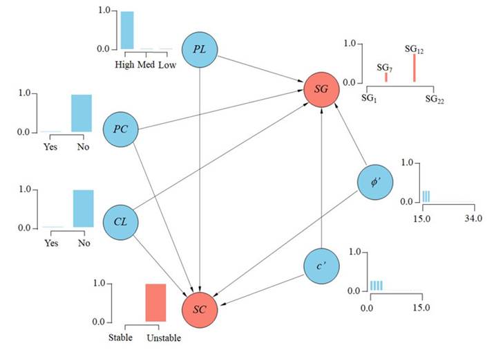
Figure 11: Updated nodes for a predictive query associated with H4 (drained condition)
When the BN is used for abductive reasoning, the available evidence (SC = Unstable, SG = SGl2) is better explained by hypothesis H4 than H1, H2, and H3. However, the probability of hypothesis H5 does not show a significant difference in comparison to H4. Therefore, H5 is also a reasonable explanation for the Breitenhagen levee failure.
The K-MPE algorithm was implemented to find the most probable explanations. Table V lists the K = 3 MPE for the drained soil constitutive model, along with the instantiations of the hypothesis nodes. For the drained condition, the best explanation for the levee failure is the existence of a conductive layer and low values of soil strength parameters. Interestingly, the second and third best explanations are also related to low values of c’ and φ’. None of the K = 3 MPE includes the pond connection as an explanation for the levee failure.
Table VI lists the K = 3 MPE for the undrained soil constitutive model. In this case, the best explanation is the simultaneous existence of a high phreatic level, a conductive layer, and low POP values. As with the drained condition, a pond connection does not explain the levee failure.
Table V: K=3 MPE for the drained soil constitutive model
K
PL
CL
PC
c
fi
P
1
Medium
Yes
No
4
17
4,92E-03
2
High
No
No
1
24
4,79E-03
3
Medium
Yes
No
3
18
4,76E-03
Table VI: K=3 MPE for the undrained soil constitutive model
K
PL
CL
PC
S
m
POP
P
1
High
Yes
No
0,33
0,74
20
1,49E-03
2
High
No
No
0,27
0,54
20
1,46E-03
3
High
Yes
No
0,39
0,54
0
1,44E-03
Discussion
The Bayesian Network approach presented in this study proposes a substantial advance for objectively determining the causes of levee failures. The five steps of the approach quantitatively account for credible hypotheses as causes of failure. Moreover, the collected evidence is transparently included in the process in order to draw conclusions based on probabilistic and abductive reasoning.
To date, little research has been published on the role of Bayesian Networks in investigating causes of geotechnical failures. For example, 13 propose a Bayesian-based method to update prior probabilities of failure scenarios by including collected evidence. However, said approach does not account for multiple or simultaneous causes due to assumptions related to mutual exclusivity in probabilistic analysis. The BN approach overcomes this limitation by assigning a node to each credible hypothesis without restricting the simultaneous occurrence of two or more events.
Other approaches, such as the ones proposed in 10, use BNs to diagnose the causes of failures based entirely on data. The probability relationships (i.e., CPTs) are learned from data without resorting to physical-based models. Although this approach could reach reasonable conclusions, data from failures is scarce and is not always available. The BN approach overcomes these shortcomings by building probability relationships via mathematical models broadly accepted by the geotechnical community.
In this work, the BN approach was applied to the Breitenhagen levee. The results demonstrate the capabilities of BN to draw conclusions about the causes of failure. The most probable explanation seems to be the simultaneous existence of a high phreatic level, a conductive layer, and low soil resistance values. Not surprisingly, this conclusion appears to agree well with previous studies based on sensitivity analysis 12 and traditional forensic analysis 11. However, the results contradict the findings of 13, which associate the failure with high pore pressures due to a pond connection to an aquifer.
The levee failure assessment using the BN approach is based on several assumptions. For instance, independence between hypothesis nodes is assumed, even though it is known that some soil parameters are correlated. Furthermore, some hypothesis nodes associated with pore water pressures could not be independent in the sense that, for example, a pond connection to an aquifer could lead to a reduction in the phreatic level. In that case, an edge between the two hypothesis nodes should be included. The results obtained from step 4 were used to confirm the independence of the hypothesis nodes. In this case, several BN structures were built using only data obtained from simulations. The best-rated BN structures did not show a correlation between the hypothesis nodes.
Another assumption is that the hypothesis nodes are collectively exhaustive. In other words, the BN encompasses the entire range of possible causes leading to failure, and at least one of them must occur to explain the failure. Other possible causes could be disregarded if they are not included in the BN. Hence, credible hypotheses should be proposed using engineering expertise.
The steady-state condition assumed for pore water pressures is a significant limitation that could lead to erroneous conclusions about the causes of failure 13. For the Breitenhagen levee failure, the pond connection seems to be irrelevant due to the high impact of the phreatic line position. The three most probable explanations derived from the K-MPE metric corroborate this assumption when comparing their probabilities of occurrence. However, unsteady conditions for piezometric pressures could be relevant. Further research studies could evaluate the influence of transient flow and assess the statistical significance between different failure scenarios using metric criteria such as the Bayes factor or the log likelihood function.
Data from slope stability simulations are used to elicit the CPTs. In this study, the limit equilibrium method and drained/undrained constitutive models (Mohr-Coulomb and SHANSEP) are used. Although finite element methods and unsaturated soil constitutive models could better represent the actual condition of the levee, the computational cost is considerably higher. Consequently, analysis methods and constitutive soil models should be selected based on accuracy requirements, the engineers experience, and available evidence.
The proposed BN approach can be generalized to any type of forensic geotechnical assessment, including but not restricted to failures in dams, slopes, foundations, and excavations. The results from this study demonstrate its capability for drawing objective conclusions about the causes of geotechnical failures.
Conclusions
A straightforward Bayesian Network approach to support decisions in forensic geotechnical engineering is presented. The approach follows a five-step sequence that reflects the generic forensic engineering process for failure assessment. Furthermore, it includes the mathematical consistency of Bayesian Networks. BNs can significantly improve the accuracy and transparency of forensic conclusions by supporting their findings on probability and abductive reasoning.
Unlike traditional forensic approaches, competing hypotheses about the causes of failure can be probabilistically compared. Besides, BNs can simultaneously deal with multiple hypotheses and find the most probable explanation to geotechnical failures.
The BN approach is applied to investigate the causes of the Breitenhagen levee failure. Three failure scenarios related to pore water conditions and two soil constitutive models with their corresponding parameters are used as hypotheses about causes of failure. Causal connections between hypothesis nodes and evidence nodes are defined through a mathematical model and common geotechnical idioms. In the case under study, the CPTs were estimated from thousands of slope stability simulations using the states of hypothesis nodes. Evidence collected from failure was used to update the BN through predictive and abductive queries.
The three most probable explanations for the levee failure were estimated using the K-MPE algorithm. A high phreatic level combined with a conductive layer and low soil strength parameters seems to be the most probable cause of failure.
The BN approach can be applied in any forensic geotechnical assessments where several competing hypotheses need to be evaluated. However, the computational effort and time required for calculation could limit its use. Future work should prioritize: 1) building efficient BN structures for describing forensic assessments and 2) extending the BNs approach to analyzing geotechnical failures in foundations, excavations, slopes, and dams.
References
License
Copyright (c) 2022 William Mauricio Garcia-Feria, Julio Esteban Colmenares Montañez, German Jairo Hernandez Perez

This work is licensed under a Creative Commons Attribution-NonCommercial-ShareAlike 4.0 International License.
![]()
From the edition of the V23N3 of year 2018 forward, the Creative Commons License "Attribution-Non-Commercial - No Derivative Works " is changed to the following:
Attribution - Non-Commercial - Share the same: this license allows others to distribute, remix, retouch, and create from your work in a non-commercial way, as long as they give you credit and license their new creations under the same conditions.

2.jpg)