Ingeniería, 2001-00-00 vol:6 nro:1 pág:51-60

---

Framing ATM Cells for Satellite Onboard Switching

Marco A. Alzate

Abstract

In this paper we analyze a simple model to study the convenience of grouping ATM cells into frames before transmission over satellite channels for onboard switching. We consider a switch where the input/output ports are mapped to the spot beams of the satellite, with several Bernoulli users within each spot beam. We obtain exact results for the delay in the terrestrial multiplexing system, based on the grouping of states of a Markov chain into equivalent cost classes. Then we obtain an approximate solution for the onboard switch delay, based on a search algorithm of the most probable states in an infinitesate Markov chain.

By using this kind of framing we reduce the number of switching operation per unit time, so we can use smaller and lighter onboard switches. However, although we also reduce the contention for accessing the uplink channel, this reduction cannot always compensate for the additional delay we incur during the framing process.

Index Terms: ATM-over-satellite, Most probable states, Performance bounds.

---

I. INTRODUCTION

THERE are many reasons to interconnect satellite and ATM networks, mainly the possibility of very fast deployment of large-scale broadband services over wide geographical areas. However, several problems arise that prevents a seamless integration of these two technologies. For example, the cell transport method should be adapted to the burst error characteristics of satellite links, which are very different to those of fiber optic; the link access schemes should be optimized for ATM technology; more elaborate traffic management procedures are necessary in order to maintain the QoS of ATM connections over satellite channels; etc.[1].

Several of these problems can be better dealt with if we allow for onboard processing. In fact, the requirement of inexpensive and small user terminals has been satisfied by the use of multiple beams, which suggests the possibility of some form of switching between beams. Of course, the space environment imposes several constraints to the onboard switches, which should be added to the typical system requirements found in terrestrial networks. These constraints include, mainly, lightweight to meet the size, mass and power limitations of the satellite, and increased fault tolerance to meet the expected life reliability of the satellite [2].

For all these reasons, it has been asked if terrestrial ATM cells should be grouped into frames before transmission over satellite channels for onboard switching [3]. In effect, if each user sends its cells directly to the satellite, the contention will work in a cell basis as well as the onboard switching operations, i.e., one contention and one switching operation per cell slot. But if we form clusters of users within each spot beam, grouping their cells into frames according to their destination and sending these frames to the satellite, then the number of contenders, the number of contentions and the number of switching operations will be reduced. Furthermore, such framing process can be easily implemented with current ATM-satellite multiple access schemes such as MF-TDMA.

In this report we consider an onboard switch where the input/output ports are mapped to the spot beams, with several Bernoulli users within each spot beam. To compare the framing concept with direct cell transmission we propose a very simple model and find approximations for the average delay. These approximations can be made arbitrarily close to the actual delay with a tradeoff between accuracy and computational cost.

The paper is organized as follows. In the second part we describe the multiplexing system and the mathematical model. In the third part we develop a performance analysis on this model, which leads to approximate results on the average delay. After some numerical results, we give some conclusions and describe the additional work to be done. An important result is proved in the appendix.

II. THE MULTIPLEXING SYSTEM

We consider a satellite communication system that uses an onboard switch in which the input/output ports are mapped to the spot beams of the satellite, where there are several Bernoulli users competing for the uplink channel access.

If each user sends its cells directly to the satellite, there will be a contention every cell slot among those users that have pending cells in that cell slot. Also, the satellite switch must work in a cell basis, i.e., it must switch each cell independently of the others. This would require a very fast switch, with corresponding implications on mass, size and power consumption.

If we form clusters of users within each spot beam, grouping their cells into frames according to their destination and sending these frames to the satellite, then the number of contenders will be reduced since now contention will not be among users but among clusters within each spot beam. Also the number of contentions per unit of time will be reduced if the frames are not transmitted at every cell slot but at longer frame periods. And, most important, the number of switching operations per unit time will also be reduced because of the longer frame periods and because switching the first cell of a frame will be enough to switch all the cells of that frame. This would require a simpler and slower switch, but can have a negative impact on the QoS parameters of the ATM connections.

Since we are interested in comparing these two alternatives regarding the grouping of cells into frames, we pay no attention to other aspects of the multiplexing systems. In particular, the onboard switch gets the arriving cells directly to their output port queues with no blocking nor delays. We do not even consider propagation delays.

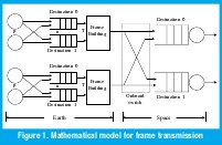
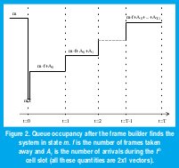
For the mathematical model, we consider two output ports and two users at each spot beam trying to access these ports. The sources are iid Bernoulli processes, each one generating one cell per slot with probability p. The destination of each cell is selected independently and equally likely. Within each spot beam there is a frame builder as well as two separate buffers for each kind of cells. The frame builder looks at these queues every T slots. If at least one of the queues has n or more cells, a frame is constructed with up to T cells taken from the longest queue. Otherwise, no frame is constructed. The frames are sent through the uplink to their corresponding output port with no switching overhead, where they are served at a rate of one cell per slot (Figure 1).

Looking at the system at frame periods of T cell slots we find an embedded Markov chain whose state is given by the lengths of each of the six queues, as seen by the frame builders. In effect, given the current state, the next state will depend only on the number of arrivals to each terrestrial queue during the next frame period, which is a tetradimensional random vector, independent from past and future arrivals. However the huge cardinality of this Markov chain makes it very difficult to carry out an exact analysis of this model, so we will also look for approximations. These approximations can be made arbitrarily close with a tradeoff between accuracy and computational cost.

In the next section, the doubly infinite state space cardinality of the terrestrial queues is reduced by the systematic approach for the construction of bounds presented in [4]. Furthermore, this approach will lead us to an exact solution obtained from the analysis of a much simpler system.

Notice that the satellite queues are deterministic servers fed with batch arrivals occurring during the phase transition of a multidimensional Markov chain of infinite cardinality in each dimension, for which the bound construction approach of [4] is not easily applied. Several authors have solved similar models under a finite number of states in the modulating chains. For example, [5] analyzes a discrete-time DBMAP/D/1/K system very similar to ours but with finite queues, and [6] analyzes a BMAP/D/1 system.

Our approach will be to look for a typical set of states of the terrestrial queues, so that we can compute the joint probability of a sequence of arrivals to a satellite queue. It comes out that the correlation between current and past arrivals to the satellite decays very quickly with time. Consequently, we consider only a few terms of this correlation by assuming that the arrival process to a satellite queue is an order-n Markov chain. Next section contains the corresponding details.

III. Performance Analysis

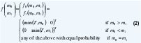
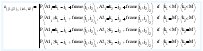
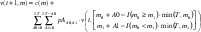
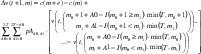
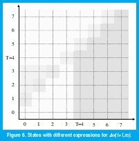
Consider the system at frame periods of T cell slots. The state of the system at time t, m(t), is given by the lengths of the queues as seen by the frame builder at the beginning of the t_th frame period (a 6Dimensional vector). For a state m, let m₀ and m₁ be the length of the queues at spot beam 0, m₂ and m₃ be the length of the queues at spot beam 1, and m₄ and m₅ be the length of the queues at the output ports. So we get a Markov chain in which the one step transition probability from state m to state µ is given by

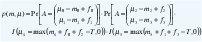
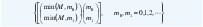
where Pr[A = (A₀ A₁)^T] is the probability that there are A₀ destination 0 arrivals and A₁ destination 1 arrivals in a spot beam during T cell slots, (f_i,f_i+1) is the number of cells taken by the frame builder from the terrestrial queues when it finds (m_i,m_i+1) cells in them, for i=0 or 2, and I(x) is the indicator function of the event x.

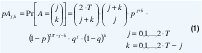
The arrival probability above is easily found to be

Note that the terrestrial processes within each spot beam are identical and independent, so we can analyze just one of them. In fact, given a sequence of states of these subsystems, the output port behavior becomes completely deterministic.

In analyzing the frame building subsystem, we will focus on the cases n=1 (when the frame builder constructs a frame whenever it finds that the queues are not both empty) and n=T (when the frame builder constructs a frame only if it can take exactly T cells away).

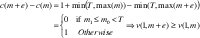
In the first case, the number of cells taken away by the frame builder when it finds (m₀, m₁) cells in the queues is

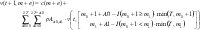
And the one-step transition probability between states (j₀,j₁)^T and (k₀,k₁)^T is

This is a tetradimensional infinite array, which implies it is very difficult to solve for the stationary distribution. However, following [4], we can find bounds for the performance measures of interest.

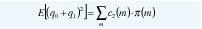
Consider, for example, the average number of cells in the queues. Let c(m) be the average number of cells in both queues during a frame period that begins in state m and let us call it "the cost of state m". If π(m) is the equilibrium probability mass function corresponding to transition probability (3), then the average number of cells in the subsystem is

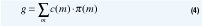
To compute g we need the cost c(m) and the probability p(m) of each state m. From Figure 2 we see that the first quantity is

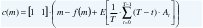
where f(m) is given by (2) and A_t is the number of arrivals during the t^th cell slot. Taking out E[A_t]=[p p]^T from the sum, evaluating the resulting sum as (T+1)/2 and carrying out the vector multiplication we get

We still need p(m) to evaluate (3), but it is not easy to obtain this exact distribution, so we construct bounds for g by modifying the state transitions as explained next [4].

A. The Terrestrial Queues

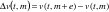
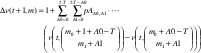
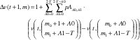
Consider the average total cost over a time interval of t frame periods starting in state m, v(t, m), i.e.,

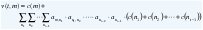
where a_m,n is the one step transition probability given by (3). Notice that this expected cost can be recursively defined as

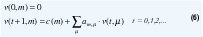
Also note that, assuming ergodicity, the average number of cells in the system, given by (4), can be expressed almost surely as

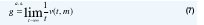
for any recurrent state m.

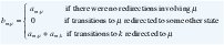
Always following [4], we say that state m has precedence over state µ (or that µ is more attractive than m, or that (m,µ) is a precedence pair, or that m→µ) if v(t,m) ≤ v(t,µ) for all t ≥ 0. The bounds we are looking for will be obtained by introducing some modifications to the original system so that, in some states, we redirect some (or all) of the outgoing transitions. For example, if we redirect all the transitions leading to state k as transitions leading to state j, the new system will have the same one-step transition probabilities of (3), b=a, except for {b_mk=0, b_m,j=a_m,k+a_m,j | for every state m}.

Now assume that all transition redirections are made between precedence pairs (j,k), i.e. we are redirecting to more attractive states. We want to prove that, in this case,

for every t=0,1,2,... and every recurrent state m in the modified system, where v_b(t,m) is the corresponding expected cost of t frame periods starting in state m for the modified system.

In effect, inequality (8) holds for t=0 since both costs are zero. Now we show that, if it holds for t, it also holds for t+1. By the recursion (6) and using the hypothesis, we get for the modified system

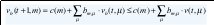
But notice that

so the above inequality becomes

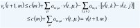
where {(j,k)} are the precedence pairs for which we made the transition redirections. The second inequality above comes from the fact that v(t,k)≥ v(t,j) since j is more attractive than k. This proves (8).

The importance of (8) is that, from (7), we get

So, if the modified system is easier to analyze than the original one, we can compute a lower bound for the average number of cells in the terrestrial queues.

In an identical way we can prove that if we redirect some transitions to less attractive states, the corresponding average number of cells will constitute an upper bound for g.

Notice that if we redirect some transitions to equivalent states (j ↔ k), we obtain a modified system that has exactly the same average cost of the original one, g=g_b. We will use this property to obtain exact values of the terrestrial queue lengths.

An Arbitrarily Tight Lower Bound For n=1

Let e=(1 0)^T. In the appendix we prove that, for n=1, the state m is more attractive than the state m+e, i.e., m→ m+e. Using symmetry and transitivity,

In particular, for some M>0,

is a set of precedence pairs. So, by truncating the queues at a maximum length of M cells, the average number of cells in the truncated system is a lower bound for the average number of cells in the original system. And since we get a finite number of states, we can easily solve this truncated system. Also notice that, making M larger and larger we are getting closer to the original system, so this lower bound can be made arbitrarily tight (with a penalty in the computational cost, of course).

Notice that truncating the queues at length M modifies (3) as follows:

Since now we have a finite number of states, (M+1)², we can reindex them to convert the above tetradimensional array into a matrix and solve for the equilibrium distribution.

An Exact Solution For n=1

We postulate the following equivalencies:

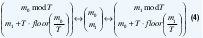
Proof. The second equivalence comes from the first one by symmetry. To prove the first one, it is enough to prove the equivalence between (m₀, m₁)^T and (m₀+T, m₁-T)^T for m₁≥T, since the iterated application of this equivalence leads to (9). For m₁≤m₀+2T the result is immediate since both states will leave the queues in (m₀, m₁-T)^T (we are assuming m₀≤m₁, without loss of generality). In effect, from (5), notice that the cost of the sate m depends on how many cells does the frame builder leave in the queues when it finds them in the state m. Accordingly, all states that leave the system with the same number of cells at each queue become equivalent since, by a simple coupling argument, they will behave identically under the same sequence of arrivals. For m₁>m₀+2T we proceed as in the appendix. Notice that the equivalence of states leaving the system with the same number of cells at each queue implies that {(m ₀,m₁) ^T ↔ (0,m₀+T)^T, m₀≤m₁≤T}, since those states leave the system with (0,m₀)^T cells, and {(0,m₁)^T ↔ (0,0)^T, m₁ ≥ T}, since those states leave the system empty.

With these equivalencies we can construct a tractable system that has an average cost exactly equal to the average number of cells we are interested in. In effect, if we redirect all transitions to (µ₀,µ₁)^T as transitions to (m₀, m₁)^T given by (10) below, we will get the same average t-frame-period cost for every t ≥ 0. So the average cost of the modified system becomes the average number of cells in the original system.

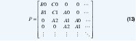
Adding a few dummy transient states, these redirections lead to a system of «quasi-birth-death» type, where the transition probability matrix is a block tridiagonal one of the form

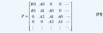
The blocks A0, A1, A2, B0 and B1 are T(T+1)/2-square matrices, so we have reduced one of the dimensions of the state space from infinity to T(T+1)/2. Although the solution can be obtained using moment generating functions, the matrixgeometric approach gives an easily implementable algorithmic technique to find the steady state distribution of the modified system and, consequently, its average cost.

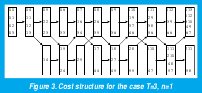
Other Bounds For n=1

Putting together the equivalence relations (9) and the precedence relations (m,m+e), we get a rich cost structure to build upper and lower bounds for g. Figure 3 shows such structure for the case T=3, n=1.

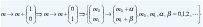
For example, we can eliminate one of the queues as follows. If (m₀,m₁)^T has an equivalent state of the form (0, µ₁)^T, we can redirect the transitions to (m₀, m₁)^T as transitions to (0, µ₁)^T without altering the average cost. Otherwise, it has an equivalent state of the form

{(µ₀, µ₁)^T: 0 < µ₀ < T , µ₁ = kT + b, µ₀ b < T , k = 1,2,3,...}

for which the cost structure above gives us following precedence pairs

(0, µ ₀ + kT )^T → (µ ₀ , kT + b )^T → (0, µ ₀ + (k + 1)T )^T

Consequently, redirecting transitions to (m₀,m₁)^T as transitions to (0,µ₀+kT)^T will give us a lower bound on g, while redirecting them to (0,µ₀+(k+1)T)^T will give us an upper bound. These bounds are easier to evaluate since the corresponding blocks of the canonical form (11) are only T-square matrices. However these bounds can become loose under very heavy loads.

An intermediate state to which we can redirect those transitions is (0, µ₀+kT+b)^T. This modification will give us an approximation since it is something between a lower and an upper bound. In fact, notice this modified system corresponds simply to the case q=1 in which we have a single queue: except for the boundary conditions in which the modified transitions are to equivalent states {(m₀,m ₁) ^T ↔ (0,m₀+T)^T, m₀ ≤ m₁ ≤ T} and {(0,m₁)^T ↔ (0,0)^T, m₁ ≤ T}, all transitions to other states (m₀,m₁)^T are redirected to (0,m₀+m₁)^T. Consequently we expect it to give us a tighter lower bound on g. In effect, although the relationship v(t,(0,kT+b+µ₀)^T) ≤ v(t,(µ₀,kT+b)^T) does not hold for every t≥0, we can verify that this inequality holds for every t large enough, which supports our intuition in the light of (7).

Although this modification leads only to an approximation (a lower bound, in fact), its computational cost is much less than the exact solution we found before since the corresponding blocks of the canonical form (11) are of size T instead of T×(T+1)/2. This is advantageous since the bound is tight enough for practical purposes.

Bounds On Other Performance Measures

We have established a set of precedence pairs (m→µ) for the cost function (5), with which we found upper and lower bounds for E[q₀+q₁], the expected number of cells in the queues. This set is the same for every cost function c for which c(m) ≤ c(µ) [4]. Consider, for example, the following cost function

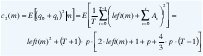
where left(m)=m ₀+m ₁-min(T,max(m ₀,m ₁)) is the number of cells left by the frame builder in the queues when it finds them in state m and A_s is the number of cells that arrive to the queues during the s^th cell slot of the next frame period.

So, using the same system modifications as before, we can also find the exact value and upper and lower bounds for

and, consequently, for the variance of the number of cells in the queues.

Case n=T

In this case, it is enough to prove that (m₀, m₁)^T ↔ (m₀+T,m₁-T)^T for m₁≥T, m₁≥m₀ in order to prove that (9) still holds. This can be done by induction as before.

On the other hand, since all states that leave the system with the same number of cells at each queue become equivalent (by a simple coupling argument, they will behave identically under the same sequence of arrivals), we also have that {(m₀, m₁)^T ↔ (m₀, m₁+T)^T , m₀<T, m₁<T}.
By these equivalencies, if we redirect all transitions to (µ₀,µ₁)^T as transitions to (m₀, m₁)^T given by (12) below, we will get the same average t-frame-period cost for every t≥0 of the original system and, consequently, the average cost of the modified system is exactly the average number of cells in the terrestrial queues.

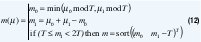
Adding a few dummy transient states, these redirections lead to a system with a block tridiagonal transition probability matrix of the form

where the blocks A0, A1, A2, B0, B1, C0 and C1 are T(T+1)/2-square matrices. The matrix-geometric approach gives an easily implementable algorithmic technique to find the steady state distribution of the modified system and, consequently, the average number of cells in the queues of the original system.
Unlike the case n=1, it is difficult to find a rich cost structure for n=T. For example consider the case n=T=2 and the states (0 1)^T and (100 100)^T. At a very low arrival rate p≅0, starting in the first state will keep one cell in the queues forever making g=1, while starting in the second state the queues will be emptied after 100 frame periods, making g=0. However, it is easy to see that truncating the queues at a multiple of T cells we get a lower bound, i.e., there is a precedence relation {(kT kT)^T → (kT+α kT+β)^T,α≥0, β≥0}. To prove this, by the previous equivalencies, it is enough to prove that {(0 kT)^T → (α kT+β)^T, 0≤αT, β≥α}, which is easily done by induction as before.

Again, making M=kT larger and larger, we are getting closer to the original system, so this lower bound can be made arbitrarily tight.

B. The Satellite Queues

Each of these queues is a deterministic server with batch arrivals occuring during the phase transition of a tetradimensional Markov chain. With an infinite number of states in each dimension of the Markov chain, there is no known solution for this system.
However we can use another arbitrarily close approximation. Assume we know the steady state pmf of the terrestrial queues as seen by the frame builder, π_i,j, so that we can compute the following sequence of conditional probabilities:

ρ_i = Probability of i cell arrivals in one frame period, i=0,1,2,,2T.

ρ_i,j= Probability of j cell arrivals in one frame period, given that there were i cell arrivals in the previous frame period, i,j = 0,1,2,,2T.

ρ_i,j,k = Probability of k cell arrivals in one frame period, given that there were a sequence of (i,j) cell arrivals in the previous two frame periods, i,j,k = 0,1,2,...,2T.

...

If in each case we ignore dependencies of higher order, we are approximating the arrival process to an r-order Markov chain: In the first case, we get independent arrivals, so the state of the satellite queue (as seen by the frame builder) is a very simple Markov chain. In the second case, the arrivals form a Markov chain so the current arrival and the current queue length form a bidiminesional markov chain. In general, if we approximate the frame arrival process as a r-order Markov Chain, the previous r-1 arrivals, the current arrival and the current queue length form a (r+1)-dimensional Markov Chain. Renumbering adequately each state, we could construct a transition probability matrix suitable again for matrix-geometric algorithmic solution techniques and, hopefully, we would notice that the autocorrelation of the arrival process decays so quickly that a second order Markov chain is a close enough model to use.

But, of course, we do not know the steady state pmf of the terrestrial queues. However, consider again the terrestrial multiplexer. Evidently, the transitions between states have highly unbalanced probabilities, i.e. it is unlikely to go to a state in which one of the queues is empty while the other one is highly occupied. In other words, within the huge state space, only a relatively small number of states account for most of the probability. If we can select a typical set of states for the terrestrial queues, we will be able to obtain a finite pmf that accurately represents the true distribution of the length of the queues. Consequently, we will be able to analyze the satellite queues as suggested above. In what follows, we will propose a dynamic search procedure to find a set of states that accounts for 100(1-δ) % of the probability, for any given small d. It is a simplified and more efficient version of the procedure in [7].

To simplify the notation, we enumerate the possible states of the system so that to the state (m₀,m₁) we associate the index 1+m₀+(m₁+m₀)*(m₁+m₀+1)/2. Conversely, we can recover the state from the index with a simple algorithm: x=floor((sqrt(8·index-7)-1)/ 2); m₀=index-(1+x·(x+1)/2); m₁=x-m₀. From now on, we will use integer numbers to specify, without ambiguities, the states of the terrestrial queues.

At step h of our dynamic procedure we have selected h states in our reduced model, Ω^<h>. Associated with this set is the set L^<h> of states that are not in Ω<h>, but through which we can leave Ω^<h>. This is, there are some states in Ω^<h> with transitions outside Ω^<h>, and L^<h> is the set of states to which those transitions are directed. We have included in our model all transitions within Ω^<h> and from Ω^<h> to L^<h>, but we still do not have transitions from L^<h>.

Now we conduct the following experiment: Starting at the initial state Ω(1) -the one we choose to initialize Ω^<1>-, we generate a sequence of states within Ω^<h> until we leave W^<h> and we register the state j in L<h> through which we leave Ω^<h>. If we repeat the experiment t times, we can measure the number of times we leave through each state j of L<h>, t_j. In the limit as the number of experiments go to infinite we get the probability of leaving Ω^<h> through state j∈ L^<h>.

Since at the end of each experiment we restart from the original initial state, we can realize an infinite number of experiments by analyzing the following Markov chain:

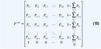
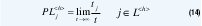
where P_i,k is the probability of going from the i^th state in Ω^<h> to the k^th state in Ω^<h> and 1-∑_k=1..h P_i,k is the probability of leaving Ω^<h> by going from the i_th> state in Ω^<h> to any state in L^<h>.
Let π^<h> = [π₁ π₂ π₃ ... π_h π_h+1] be the steady state solution to the above Markov Chain. Then PL_j^<h> can be computed easily as

where P_{Ω (i),L(j)} is the transition probability from the i^th state in Ω^<h> to the j^th state in L^<h>.

The (h+1)^st state to be included in the Typical set Ω is the one that maximizes PL, i.e. we find

then move the corresponding state from L to Ω and update L, i.e.,

Ω^{<h +1>} = Ω^<h> ∪ {L^<h> (k)}
L^<h+1> = {L^<h> ∩ {L^<h> (k)}^c} ∪ {Neighbors of L^<h>(k) not in Ω ^<h+1> }

C

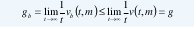
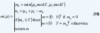
The algorithm terminates when the last element of π^<h> is less than or equal to , in which case the probability of remaining in Ω^<h> is 1-δ.

Notice that, to find h states, we need to solve h Markov Chains of increasing size from 2 to h+1. However, we do not need to invert any matrix because we can use the previous π as an approximation for the next π and solve each Markov Chain iteratively.

Once we have selected the states to be included in our simplified model, we can block the arrivals that lead to a non-typical state. This is a special kind of a truncation model that, according to the results of section III(A), leads to a lower bound on the buffer occupancy. Of course, adding more states we can obtain a better approximation.

Using this specially truncated model, the satellite queues become a discrete-time batch Markovian arrival process served by a deterministic server (a D-BMAP/D/1 system [5]). In effect, the two earth stations form a discrete-time Markov chain and, at each phase transition of this chain, a batch of size equal to the sum of the length of the frames with destination 0 arrive to the queue of the output port 0. The size of the batch is a random function of the phase of the modulating chain (f₀(m₀,m₁) + f₀(m₂,m₃), which is deterministic when m₀≠m₁ and m₂≠m₃, but it is random when m₀=m₁ or m₂=m₃). In [5] there is an analysis of a similar system modeling a source of VBR video. However, in this special case, as explained before, the autocorrelation function of the frame arrival process decays so fast that it is enough to consider only a first or second order term to obtain highly accurate results.

IV. NUMERICAL RESULTS

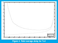
The total delay of a cell in the whole system is the sum of the delay in the earth station and in the output port of the satellite, as appreciated in Figure 4.

Figure 5 compares the multiplexing system (with n=1), for different values of T, against the cell arrival rate for the cases of direct cell transmission with TDMA, binary exponential backoff Alloha and an ideal multiple access scheme in which every cell seizes the uplink channel in strict order of arrival and with zero overhead due to contention.

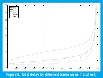
Clearly, the ideal medium access scheme is better in terms of delay than any choice of parameters of the framing system, as expected. However, for small values of T and for n=1, the figure shows a favorable performance of the framing system compared with more realistic access schemes.

The delay increases with n and T but in different ways: While an increase in T produces an overall increase in the mean delay, higher values of n affect principally (and dramatically) the light load region of the delay plot. This makes intuitive sense since, for n>1, the first cell that arrives to an empty terrestrial queue must wait, at least, the arrival of n-1 more cells to that queue before being transmitted over the uplink channel. This event can take quite a long period of time if the probability of arrivals is very small.

Also notice that, once we choose a pair of parameters (T,n), the onboard switch must be designed to be able to carry out two switching operations every T cell slots, irrespectively of the value of n. When we choose a big value for n, for example n=T, the onboard switch will be very efficiently operated, since each operation will switch T cells at once. However, this will not give any advantage if we leave the switch idle while there are cells waiting in the earth queues, in which case the QoS will be negatively impacted. Consequently, the parameter n must be chosen to be 1, i.e., the frame builder must take whatever it finds in the terrestrial queues (up to the maximum of T cells).

The parameter T should be chosen as big as possible to reduce the size, weight and power consumption of the onboard switch, as long as the impact on the average delay is acceptable for the QoS requirements. Comparing with the ideal access scheme, this condition implies that we can choose only among very small values of T. However, it seems that we can choose higher values of T if we compare the performance against more realistic access schemes. In fact, it seems possible to choose some small T with which we can obtain both benefits: a simpler onboard switch and a smaller average delay.

V. CONCLUSIONS

In this paper we presented the partial results of an ongoing work to assess the convenience of grouping ATM cells into frames before transmission over satellite channels for onboard switching. We analyzed a simple model that captures the advantage of requiring a smaller onboard switch and shows that the price that we must pay for such benefit is an increase in the average cell delay. However it seems possible to choose the main parameter T so as to compensate the increase in the delay with the reduction of contention for channel access, in which case the framing of ATM cells will be more plausible.

We also observed how important it is to attend any backlogged traffic at each frame period, even if the payload of the corresponding frame is just a single cell (i.e., choosing the parameter n to be 1). Otherwise we can introduce an unnecessary high delay under light traffic, without obtaining any apparent benefit.

We used the interesting cost structure approach of [4] to obtain exact analytical results for the average delay in the terrestrial queues. However, such method did not allow us to compute the steady state pmf of the terrestrial queue lengths, which is necessary to obtain accurate results on the satellite buffer occupancy. To this purpose, we developed a dynamic procedure to obtain a set of typical states, one which accounts for the (1-δ)100% of the whole probability. With this finite set we computed some conditional probabilities on the cell arrival process to the satellite queues. Based on the fact that the autocorrelation function of these sequences of arrivals decays so fast with time that we can consider only a few of its first terms, we computed a very close approximation to the delay in the satellite buffer.
With the methods above we can consider a more general model for the input traffic that allows a better representation of the effects of the reduced contention. For example, we should consider a bigger number of users grouped into clusters with contention among clusters. We should also measure additional performance parameters (specially the overflow probabilities) to consider the special problems of guaranteeing a given QoS for ATM over satellites.

APPENDIX

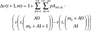
In this appendix we prove that, for n=1, m → m+e, where e=(1 0)^T. Notice the condition for precedence holds for t=1

Now assume v(t,m+e)≥v(t,m) holds for some t (we have just shown it holds for t=1). We want to show that this implies v(t+1,m+e)v(t+1,m). From (6), the corresponding average costs for t+1 frame periods are

and

where A0 is the number of destination 0 arrivals and A1 is the number of destination 1 arrivals during one frame period. If we define the difference

then what we want to show is that

For any state m we have

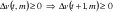
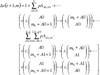
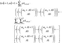
We will rewrite this expression for 6 different cases, as shown in figure 6.

Case 1: m₁ ≤ m₀ < T In this case c(m+e)=c(m) and v(t,m+e+A-f(m+e))=v(t,m+A-f(m)) so Δv(t+1,m) is zero.
Case 2: m ₀ ≥ max(m₁, T ) In this case (9) becomes

which is greater than or equal to 1 since, by hypothesis, the difference of costs within the sum is nonnegative.

Case 3: m₀ + 1 < m₁ < T In this case (9) becomes

which is also greater than or equal to 1 by hypothesis.

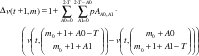
Case 4: m₁ max(T, m₀ + 2) In this case (9) becomes

which is also greater than or equal to 1 by hypothesis.

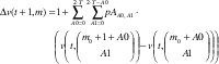
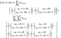
Case 5: m₀ + 1 = m₁ < T In this case (9) becomes

To verify that this quantity is always positive notice that, from (1) we get pA_A0,A1 = pA_A1,A0, so we can factorize these terms in the above sum yielding

By symmetry we know that v(t,(m₀ m₁)^T) = v(t,(m₁ m₀)^T). Applying this reversing in some costs above we get

which is greater than or equal to 1 by hypothesis.

Case 6: m₀ + 1 = m₁ ≥ T In this case (9) becomes

Using the same factorization and reversing of Case 5, we get

which is also greater than or equal to 1 by hypothesis.

REFERENCES

[1] I. Akyildiz and S. Jeong. "Satellite ATM Networks: A Survey", IEEE Communication Magazine, July 1997, pp. 30-43.

[2] J. Gilderson and J. Cherkaoui, "Onboard Switching for ATM via Satellite", IEEE Communication Magazine, July 1997, pp. 6670.

[3] M. Krunz, A. Makowski, P. Narayan and E. Slud. "Traffic Modeling and Performance Evaluation Methodologies for High Performance Networks", A proposal to the National Science Foundation, January 1998.

[4] G. van Houtum, W. Zijm, I. Adan and J. Wessels. "Bounds for Performance Characteristics: A Systematic Approach via Cost Structures", Commun. Statist. ­Stochastic models, 14(1&2), 205224 (1998).

[5] C. Blondia and O. Casals. "Statistical multiplexing of VBR sources: A matrix-analytic approach", Performance evaluation 16 (1992) 5-20. North Holland.

[6] M. Neuts. "Matrix-Geometric Solutions in Stochastic Models", Dover Publications, New York, 1981

[7] Dragomir D. Dimitrijevic and Mon-Song Chen. "An Integrated Algorithm for Probabilistic Protocol Verification and Evaluation" IEEE Infocom 1989, pp. 69-73.

[8] Iera, A., Molinaro, A. and Marano, S. "Managing Data Traffic in Integrated Terrestrial and Satellite Systems", IEEE Personal Comm. April 2000, pp. 56-64.

[9] Hsing, T., Cox, D., and Fung, L. "Wireless ATM", editors of the special issue of IEEE Journal on Selected Areas in Communications, January 1997.

[10] Kota, S. Jain, R. and Goyal, R. "Satellite ATM Network Architectire", editors of the especial issue of IEEE Communications Magazine, March 1999.

[11] Takis, P. and Salkintzis, A. "Satellite-based Internet Technology and Services", editors of the special issue of IEEE Communications Magazine, March 2001.

[12] Salkintzis, A. "Multimedia communicactions over Satellites", editor of the special issue of IEEE Personal Comm., june 2001.

Marco A. Alzate
Received his electronic engineering degree from Universidad Distrital, Bogotá, Colombia, in 1989 and his M.S. degree in electrical engineering from Universidad de los Andes, Bogotá, in 1991. From 1989 to 1992 he worked at the Research Division of ITEC, Bogotá and then he joined the Faculty of the Electronic Engineering Department at Universidad Distrital, Bogotá, where he is currently an associate professor. Now he is working for his Ph.D. degree in electrical engineering at University of Maryland, College Park, Maryland, under a Colciencias-Fulbright scholarship with a study commission from Universidad Distrital.

---

Creation date: