DOI:
https://doi.org/10.14483/23448393.20447Published:
2023-10-17Issue:
Vol. 28 No. 3 (2023): September-DecemberSection:
Civil and Environmental EngineeringComparative Analysis between Singular Spectral Analysis and Empirical Mode Decomposition for Structural Damage Detection
Análisis comparativo entre el análisis singular espectral y la descomposición modal empírica para detección de daño estructural
Keywords:
Hilbert-Huang Transform, Signal Analysis, Structural Health Monitoring, Time-Frequency Analysis (en).Keywords:
Transformada Hilbert-Huang, Análisis de señales, Monitoreo de salud estructural, Análisis tiempo-frecuencia (es).Downloads
References
C.-H. Loh, C.-H. Chen, and T.-Y. Hsu, .Application of advanced statistical methods for extracting long-term trends in static monitoring data from an arch dam,"Struct. Health Mon., vol. 10, pp. 587-601, Nov. 2011. https://doi.org/10.1177/1475921710395807 DOI: https://doi.org/10.1177/1475921710395807
L. Chin-Hsiung, C. Chia-Hui, and M. Chien-Hong, "Detecting seismic response signals using singular spectrum analysis,"Sensors Smart Struct. Tech. Civil Mech. Aerospace Sys., vol. 7647, pp. 535-546, 2010. https://doi.org/10.1117/12.846427 DOI: https://doi.org/10.1117/12.846427
B. Medina and L. Duque, "Fuzzy entropy relevance analysis in DWT and EMD for BCI motor imagery applications, Ing, "vol. 20, no. 1, pp. 9-19, 2015. https://doi.org/10.14483/udistrital.jour.reving.2015.1.a01 DOI: https://doi.org/10.14483/udistrital.jour.reving.2015.1.a01
E. Johnson, H. Lam, L. Katafygiotis, and J. Beck, "Phase I IASC-ASCE structural health monitoring benchmark problem using simulated data,"J. Eng. Mech., vol. 130, no. 1, pp. 3-15, 2004. https://doi.org/10.1061/(asce)0733-9399(2004)130:1(3) DOI: https://doi.org/10.1061/(ASCE)0733-9399(2004)130:1(3)
G. Gilbert-Rainer and P. Zeno-Iosif, "Modal identification and damage detection in beam-like structures using the power spectrum and time–frequency analysis,"Signal Proc., vol. 96, part A, pp. 29-44, 2014. https://doi.org/10.1016/j.sigpro.2013.04.027 DOI: https://doi.org/10.1016/j.sigpro.2013.04.027
D. Pines and L. Salvino, "Structural health monitoring using empirical mode decomposition and the Hilbert phase,"J. Sound Vibr., vol. 294, no. 1, pp. 97-124, 2006. https://doi.org/10.1016/j. jsv.2005.10.024 DOI: https://doi.org/10.1016/j.jsv.2005.10.024
N. Cheraghi and F. Taheri, .A damage index for structural health monitoring based on the empirical mode decomposition,"J. Mech. Mater. Struct., vol. 2, pp. 43-61, March 2007. https://doi.org/10. 2140/jomms.2007.2.43 DOI: https://doi.org/10.2140/jomms.2007.2.43
L. Cano, .On time-frequency analysis for structural damage detection,"PhD thesis, Univ. Puerto Rico, Puerto Rico, 2008. [Online]. Available: https://www.researchgate.net/publication/257138876_On_TimeFrequency_Analysis_for_Structural_Damage_Detection
D. Swagato and S. Purnachandra, "Structural health monitoring techniques implemented on IASC-ASCE benchmark problem: A review,"J. Civil Struct, Health Monitor., vol. 8, pp. 689-718, 2018. https://doi.org/10.1007/s13349-018-0292-5 DOI: https://doi.org/10.1007/s13349-018-0292-5
B. Basuraj , H. Budhaditya, and P. Vikram, Real time structural damage detection using recursive singular spectrum analysis,ïn 13th Int. Conf. App. Stat. Prob. Civil Eng., 2019, pp. 1-8. https://s-space.snu.ac.kr/bitstream/10371/153487/1/358.pdf
S. Sony and A. Sadhu, "Multivariate empirical mode decomposition-based structural damage localization using limited sensors,"J. Vibr. Control, vol. 28, no. 15-16, pp. 1863-2167, 2021. https://doi.org/10.1177/10775463211006965 DOI: https://doi.org/10.1177/10775463211006965
D. Yansong, S. Zongzhen, and G. Kongzheng, "Structural damage identification under variable environmental/operational conditions based on singular spectrum analysis and statistical control chart,"Struct. Control Health Monitor., vol. 28, no. 6, pp. 1-19, March 2021. https://doi.org/10.1002/stc.2721 DOI: https://doi.org/10.1002/stc.2721
J. I. Campos Hernández, Ïnnovador método para detectar daño estructural, funciones de la bifurcación frecuencial modal (modal frequency splitting functions),"Master thesis, Inst. Polit. Nac., Mexico, 2018. [Online]. Available: http://tesis.ipn.mx/handle/123456789/27096
R. Zhang, M. Asce, S. Ma, E. Safak, and S. Hartzell, "Hilbert-Huang transform analysis of dynamic and earthquake motion recordings,"J. Eng. Mech. ASCE, vol. 129, no. 8, pp. 861-875, 2003. https://doi.org/10.1061/(asce)0733-9399(2003)129:8(861) DOI: https://doi.org/10.1061/(ASCE)0733-9399(2003)129:8(861)
L. Plazas, M. A. Avila, and A. Torres, "Spectral estimation of UV-Vis absorbance time series for water quality monitoring,"Ing, vol. 22, no. 2, pp. 211-225, 2017. https://doi.org/10. 14483/udistrital.jour.reving.2017.1.a01
K. Liu, S. Law, Y. Xia, and X. Zhu, "Singular spectrum analysis for enhancing the sensitivity in structural damage detection,"J. Sound Vibr., vol. 333, no. 2, pp. 392-417, 2014. https://doi.org/10.1016/j.jsv.2013.09.027 DOI: https://doi.org/10.1016/j.jsv.2013.09.027
M. A. de Oliveira, J. V. Filho, V. Lopes, and D. J. Inman, .A new approach for structural damage detection exploring the singular spectrum analysis,"J. Intel. Mater. Syst. Struct., vol. 28, no. 9, pp. 1160-1174, 2017. https://doi.org/10.1177/1045389x16667549 DOI: https://doi.org/10.1177/1045389X16667549
J. Yang, Y. Lei, S. Lin, and N. Huang, "Hilbert-Huang based approach for structural damage detection,"J. Eng. Mech., vol. 130, no. 1, pp. 85-95, 2004. https://doi.org/10.1061/(asce)0733-9399(2004)130:1(85) DOI: https://doi.org/10.1061/(ASCE)0733-9399(2004)130:1(85)
How to Cite
APA
ACM
ACS
ABNT
Chicago
Harvard
IEEE
MLA
Turabian
Vancouver
Download Citation
Recibido: 8 de febrero de 2023; Revisión recibida: 5 de julio de 2023; Aceptado: 9 de agosto de 2023
Resumen
Contexto:
En los últimos años, gracias a los avances tecnológicos en instrumentación y procesamiento digital de señales, los métodos no invasivos para la detección de daños estructurales se han vuelto cada vez más importantes. Las técnicas de monitoreo de salud estructural (SHM) basadas en vibraciones permiten identificar la presencia y ubicación del daño a partir de cambios permanentes en las frecuencias fundamentales de las señales. Un método empleado con éxito para la detección de daño es la descomposición modal empírica (EMD). Otro método menos utilizado en este campo de estudio es el análisis singular espectral (SSA). En este artículo se describen ambos métodos y se realiza un estudio de simulación para compararlos e identificar cuál es más efectivo en la detección del daño estructural.
Métodos:
Se aplicaron los métodos de un estudio de referencia conocido como benchmark SHM problema para facilitar la comparación. Para evaluar la efectividad de ambos métodos, se empleó la simulación Monte Carlo. Para controlar el ruido aleatorio y otros factores inherentes a la simulación, se repitió el procedimiento 1.000 veces para cada tipo de daño.
Resultados:
En el caso de daño severo, ambos métodos mostraron un buen desempeño. Sin embargo, cuando el daño fue leve, los cambios en la frecuencia fundamental no fueron aparentes. Sin embargo, se observó un cambio significativo en el nivel de amplitud. En este caso, el método SSA obtuvo los mejores resultados.
Conclusiones:
Los métodos EMD y SSA, junto con el filtro de paso alto, detectaron daños severos cuando los registros de aceleración tenían poco o ningún ruido. Cuando los registros de aceleración estaban contaminados con ruido, la probabilidad de que el EMD detectara el daño disminuyó drásticamente. Una de las ventajas del SSA sobre el EMD es que, para patrones de daño moderado o leve, el primero no requiere filtros ni el uso de la transformada Hilbert-Huang para detectar el daño. En general, se encontró que el SSA es más efectivo para la detección de daño.
Palabras clave:
transformada Hilbert-Huang, análisis de señales, monitoreo de salud estructural, análisis tiempo-frecuencia.Abstract
Context:
In recent years, thanks to technological advances in instrumentation and digital signal processing, noninvasive methods to detect structural damage have become increasingly important. Vibration-based structural health monitoring (SHM) techniques allow detecting the presence and location of damage from permanente changes in the fundamental frequencies of signals. A successfully employed method for damage detection is empirical mode decomposition (EMD). Another method, less used in this field of study, is singular spectral analysis (SSA). This paper describes both methods and presents a simulation study aimed at comparing them and identifying which one is more effective in detecting structural damage.
Method:
The methods of a reference study known as benchmark SHM were applied to facilitate the comparison. To evaluate the effectiveness of both methods, Monte Carlo simulation was employed. To control the random noise and other factors inherent to the simulation, the procedure was repeated 1.000 times for each type of damage.
Results:
In the case of severe damage, both methods showed a good performance. However, when the damage was slight, the changes in the fundamental frequency were not apparent. However, a significant change in the amplitude level was observed. In this case, SSA obtained the best results.
Conclusions:
The EMD and SSA methods, together with high-pass filtering, detected severe damage when the acceleration records had low or no noise. When the acceleration records were contaminated with noise, the likelihood of EMD detecting the damage decreased dramatically. One of the advantages of SSA over EMD is that, for moderate or mild damage patterns, the former does not require filters or the use of the Hilbert-Huang transform to detect damage. In general, it was found that SSA was more effective in detecting damage.
Keywords:
Hilbert-Huang transform, signal analysis, structural health monitoring, time-frequency análisis.Introduction
General aspects
In recent decades, many researchers have paid special attention to avoiding the sudden failure of structural components through early damage detection. There are several techniques for damage analysis, including vibration-based methods. However, it is necessary to implement a time series-based algorithm to process the large amount of information provided by sensors and simplify the measurement of structural conditions.
A method that provides good results for damage detection is the Hilbert-Huang transform (HHT), which combines empirical mode decomposition (EMD) with Hilbert spectral analysis. Additionally, there is a new approach called singular spectral analysis (SSA), which has been widely employed in recent years. For example, according to 1 and 2, singularities can be associated with cracks, damage, or environmental changes. Specifically, SSA is a time-series analysis technique that decomposes the signal into specific principal components that describe its trend, fundamental frequencies, and singularity effects.
EMD and SSA allow decomposing a signal into mono-component signals (i.e., signals with a single fundamental frequency). Once the decomposition is performed, it is possible to use Hilbert spectral analysis to study the decomposed signals in the time-frequency domain and observe whether there is a change in the natural frequencies (i.e., structural damage). This is valid in a broad field of applications, such as the detection of brain damage 3.
This article compares the effectiveness of SSA and EMD in detecting structural damage based on a simulation study that applied these methods to the dynamic acceleration response of a four-story Steel structure with different damage patterns. This acceleration response was generated through a computer program called Datagen, which simulates a reference known as the benchmark SHM problem developed by the IASC-ASCE structural health research group 4.
Background
Different tools have been developed to study damage from changes in natural frequencies, with the purpose of monitoring structural health. This is associated with the mass and stiffness matrix of the structure. Generally, the mass tends to remain constant, so, if there are frequency changes, they will be caused by changes in stiffness. When this variation is longstanding, it indicates damage to the structure. For example, 5 performed modal identification and detection of damage in beam-type structures by analyzing methods based on natural frequency changes.
6 used instantaneous phase data obtained from single-component decomposition for damage detection in a three-story building. 7 proposed a damage index called the EMD energy damage index for structural damage detection, corroborating its applicability through numerical and experimental studies. 8 described the beginnings, current state of the art, and potential advances in diagnostic and damage detection analysis. They developed a new method for system identification and damage detection using actual output data from vibration records, based on the direct application of time and frequency averaging representation (MTFR) and frequency domain decomposition (FDD).
9 performed a comparative review on different damage detection methods, including ARMA models, parameter identification tools, NexT/ERA identification systems, damage indices, EMD, EMD+HHT (Hilbert-Huang transform), AR models, and others. These methods, when applied to a benchmark problem, allowed analyzing the advantages and disadvantages of each of these methods and their detection capabilities with regard to different damage patterns.
Recent research has implemented different methods for vibration-based damage detection. For example, 10 used the recursive spectral singular analysis algorithm to identify structural damage, using a single channel in real time as input, and produced a lagged Hankel time matrix of the series. This method allowed obtaining information about the current state of the structure - in this case, a cantilever beam subjected to seismic excitation. 11 proposed the use of multivariate empirical modal decomposition to locate damage in structures via measurements. 12 used EMD with adaptive noise to identify the presence, location, and severity of damage in a steel truss bridge model. They built the object of study under laboratory conditions and they experimentally subjected the bridge to white noise excitations.
9 confirmed that EMD, together with the Hilbert-Huang transform, can detect specific damage patterns. They further verified this result and implemented SSA, which is still an innovative algorithm for structural damage detection in the field of civil engineering.
Materials and methods
This section briefly explains some concepts regarding damage, as well as some mathematical concepts associated with time-frequency analysis.
Levels of structural damage
In civil engineering, the concept of damage has different meanings and interpretations. In this study, structural damage is defined as the changes (almost always permanent) in structural properties such as stiffness, strength, and dynamics, in addition to losses of acceptable structural performance according to pre-established behavior criteria 8.
The effects of damage in a structure can be classified into four levels, as follows 13:
-
Level 1 indicates the presence of damage in the structure
-
Level 2. Level 1+ determines the geometric location of the damage
-
Level 3. Level 2+ quantifies the severity of the damage
-
Level 4. Level 3+ predicts the remaining service life of the structure
Generally, vibration-based damage identification methods that do not use a structural model mainly provide level 1 and 2 damage identification.
Empirical mode decomposition (EMD)
EMD is a method for decomposing a given signal into a set of elementary signals called intrinsic mode functions (IMFs), which are defined by the following conditions 14:
1. The number of extremes (max and min) and zero crossings must not differ by more than one.
2. At any given instant, the average between the envelope of maximum points and that of mínimum points must be close to zero.
The iterative procedure proposed by Huang to obtain IMFs is as follows:
1. Identifying the extreme points of the function x(t) (max. and min.).
2. Interpolating between the maximum points using a cubic spline to obtain an envelope
.

The same is done with the minimum points to obtain
. The envelopes should cover the entire signal.

3. Calculating the average of the envelopes
.
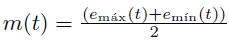
4. Calculating h(t) = x(t)−m(t) , where h(t) is the IMF candidate. Steps 1-4 should be iterated with h(t) as the new function until the two aforementioned conditions for IMFs are met.
5. Once the conditions have been met, h(t) becomes the first IMF.
6. Calculating the residue
becomes the new function, and the steps are repeated to find the next
.

7. The procedure is repeated until the residual can be considered negligible or is a monotonic function (no max. or min.).
In summary, this process is based on generating envelopes defined by the max. and min. of a series and subtracting the average of these envelopes from the initial series.
Singular spectral analysis (SSA)
This method incorporates classical time series analysis elements such as spectral analysis (15), digital signal processing, dynamic systems, and multivariate statistics. SSA consists of decomposing an original signal into a set of uncorrelated components from which three characteristics can be extracted: trend, oscillation, and noise 16,17. This decomposition is based on the Karhunen-Löeve covariance matrix. The procedure is has four steps:
Step 1: Decomposition of the time series
Let Y = {y1, y2, . . . , yN} be the observed time series with a size N. Consider the matrix X of dimension L × K given by
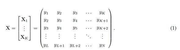
L is the length of the window, such that 2 ≤ L ≤ N, K = N − L + 1 is the number of columns in the matrix X and each Xi = (yi, . . . , yi+L−1)T , 1 ≤ i ≤ K. Choosing the length L is one of the greatest challenges when working with SSA, mainly for non-stationary series, since a large window may require higher computational efforts, and a small window may separate the noise from the trend components.
Note that X is a matrix of trajectories known as the Hankel matrix, where the component yi,j of row i and column j satisfies yi,j = yi−1,j+1 = yi+1,j−1, leading to X having equal elements over the anti-diagonals.
Step 2: Decomposition of X into singular values (SVD)
Let W = XXT be a square matrix L × L. Then, the positive eigenvalues (λ1 > λ2 > . . . > λd) of W and their corresponding eigenvectors U1,U2, . . . ,Ud are found. The square root of the eigenvalues
 of W are the singular values of the matrix X, and the corresponding eigenvectors Ui are the left singular vectors of the matrix X.
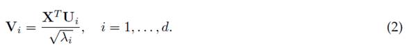
Other singular vectors computed by Eq. (2) correspond to the right singular vectors of the matrix X.
Each eigentriplet
 of the matrix X determines the corresponding components, and all eigentriplets determine a d-dimensional subspace in
 . Then,

and the matrix X can be expressed as

Step 3: Grouping the eigentriplets
This step selects the desired components from all those obtained in step 2. Usually, the selection criterion is determined a priori, which can be a problem since SSA projects the original data into different orthogonal components, but it is not easy to find all the components with the required information, given that this depends on the window length selected in step 1.
Once the expression 4 has been obtained, in this step, the set of indices is partitioned {1, . . . , d} into m disjoint subsets
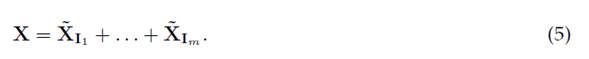
 . Then, the resulting matrix XI corresponding to group I is defined as XI = Xi1 +. . .+Xip . A matrix is calculated for each group I1, . . . , Im, and the expansión of 4 leads to the decomposition
The procedure for selecting the sets I1, . . . , Im is called eigentriplet clustering. Furthermore, a relation given by (6) can be defined, which quantifies the degree of approximation of the original signal’s windows.

Step 4: Averaging the diagonals
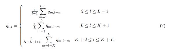
In reconstructing the required signal from the selected components, each matrix XIj of the decomposition given in Eq. (5) is transformed into a new series of length N, using the procedure for averaging over the diagonals, which defines the value of the time series as an average of the diagonals corresponding to each matrix in XIj .
This procedure is based on the following: let Q = (qi,j) be any L × K−size matrix, where each element qi,j , (i + j = l) becomes an element of Hankel’s matrix. Thus,
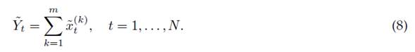
This is known as the Hankelization procedure, and applying it to all components of the XIj matrices yields a reconstructed series
 . Therefore, the initial series y1, y2, . . . , yN is decomposed into the sum of m reconstructed series, as follows:
Each component provides part of the retained energy obtained from the original series. Clearly, the larger the number of components is, the greater the information collected from the initial series. Therefore, another challenge in working with SSA is identifying the number of components to be used in the reconstruction procedure. In order to solve this problem, specific experimental tests are performed together with eigenvalue analysis in order to have better accuracy in selecting the number of components needed for the reconstruction process.
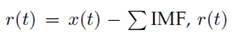
The residual rt can be calculated by considering the difference between the original and the reconstructed series, as follows:
Structural health monitoring benchmark problema
Applying different methods to different structures can generate specific difficulties when making comparisons. In this sense, the structural health monitoring research group (IASC-ASCE) developed a series of reference problems known as benchmark SHM problems, which are divided into two phases. This section details the first phase of this study, based on the simulated response of a test structure to which the two methods for damage detection were applied.
Benchmark structure
The benchmark structure is a four-story steel structure with three portal frames in each direction, 2,50 m spans, and 3,60 m floor height. The elements are made of 300 W hot-rolled steel with a nominal yield strength of 300 MPa. The sections are unusually designed for a scale model. All columns are oriented so that their strong axis is in the x-direction and their weak axis is in the y-direction, while the strong axis of the inter-story beams is in the z-direction. There are two diagonal suspenders on each floor of each exterior face, which can be removed to simulate damage. There is one floor slab per compartment: four 800 kg slabs on the first level and four 600 kg slabs each on the second and third levels. On the fourth level, there are four 400 kg slabs or three 400 kg slabs and one 550 kg slab to créate some mass asymmetry.
Through the benchmark problems, and using the finite element method, it is possible to generate a dynamic analysis in time with 12 or 120 degrees of freedom (DOF). 12 DOF restrict all motions except two horizontal translations and one rotation per floor, while the 120 DOF case has only one constraint. The nodes at the base have the exact horizontal translation and rotation in the plane. On the other hand, the columns and floor beams are modeled as Euler-Bernoulli beams, and the braces are bars with no bending stiffness 4.
The damage patterns introduced in the structure are shown in Table I and shown in Fig. 1. According to 9, the removal of braces in the story, which leads to stiffness reduction, is considered as major damage scenario and the weakening of beam column joint by loosening of bolts or reduction of stiffness for braces is considered as minor damage scenario of the structure". Therefore, severe damage patterns correspond to 1 and 2, moderate damage patterns are denoted a 3, 4, and 5, and the slight damage pattern is 6. The modeled damage patterns are predefined, and the analysis is carried out accordingly.
Table I: Benchmark problem damage cases 9
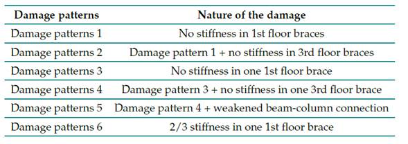
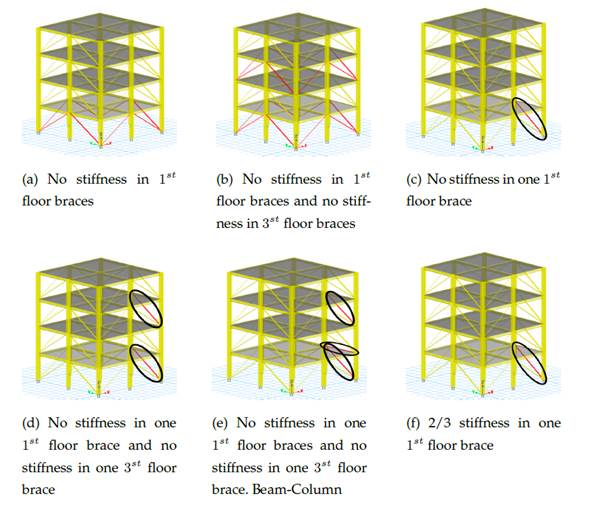
Figure 1: Damage scenarios for the benchmark structure 9
Results
Identifying damage time instants and locations
To study the sensitivity of the studied methods in detecting these damages, Table II indicates some parameters for the simulation study of the benchmark problem. The force is calculated using the FAST Nigam-Jennings method, e = 1% damping is fixed to the critical, the time step size is dt = 0, 001, and, in this case, the force intensity is F = 150. This is a constant coefficient that the program uses to calculate excitations. It also uses a filter index called Findx, a Boolean value (0 or 1) indicating whether or not the excitations should pass through a Butterworth filter (for more details, see (4)). Similarly, all acceleration records were simulated up to t = 80s. For the sake of clarity in the graphs, only 30s and 50s are shown in the figures, both for EMD and SSA.
Table II: Fixed model parameters in the simulation study
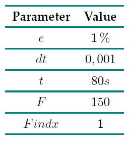
Fig. 2 shows the acceleration records of the first and second floors for damage patterns 1 and 2, respectively (without noise). To these signals, a high pass filter = 250 Hz was applied. Figs. 3aand 3b show that, on the first floor, the damage occurs at 35 s, while, on the second floor, it occurs at 40 s. It is clear from the results that, if the noise pollution is either zero or very small, the EMD method is capable of detecting the damaging time instants and locations. The same happens when applying the reconstructed components (RCs) version of SSA. Fig. 4 shows that, on the first floor, the peak occurs at 35 s and, on the second floor, at 40 s.
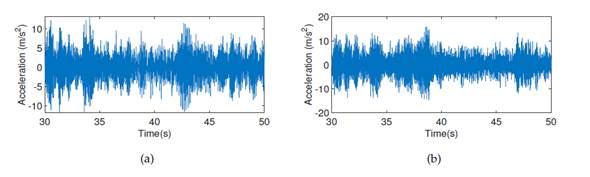
Figure 2: Acceleration records: (a) first floor, (b) second floor. All graphs correspond to damage pattern 2.
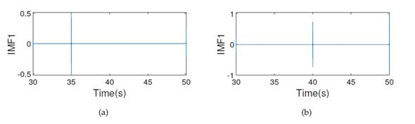
Figure 3: IMF1: (a) first floor, (b) second floor. All graphs correspond to damage pattern 2.
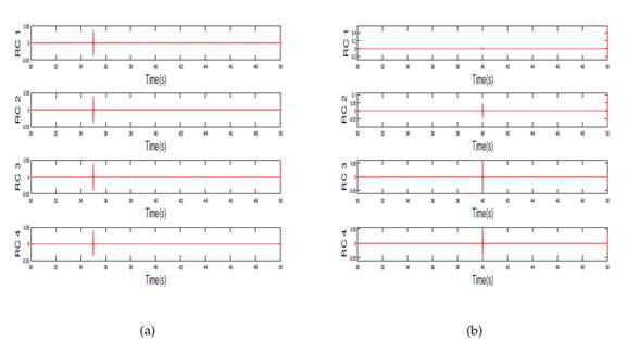
Figure 4: RCs for damage patterns 1 and 2: a) first floor, b) second floor
When the acceleration records are polluted by noise and the resulting magnitude of the damage spike is smaller than the noise levels, then the damage spike merges with the noise. For example, in Fig. 5, a signal with a noise level of 10% and damage pattern 2 was generated. This corresponds to the acceleration records of the first floor.
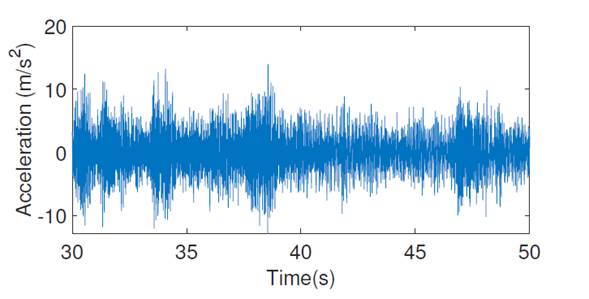
Figure 5: First floor acceleration records for damage pattern 2: sensor on the right side
It is worth mentioning that the model considers two sensors on each floor (one on the left side and the other on the right side). Therefore, there are two acceleration records for each floor. Fig. 2 only shows one acceleration record per floor, since both are identical when the structure is symmetrical and the signal is not contaminated. However, when the signal is contaminated with noise, the acceleration records of each sensor per floor are different. However, this paper only shows the sensor on the right side of the first floor, as shown in Fig. 5.
By processing the signals via EMD, the first IMF was obtained (Fig. 6) using a high pass filter = 250 Hz for the sensor signal on the right side. However, it was not possible to identify the discontinuity peak, which was confused with noise. According to 18, EMD’s ability to detect signal damage at anoise level of 10% is about 30% in the benchmark problem.
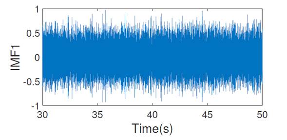
Figure 6: First IMFs for damage pattern 2 with a highpass filter: sensor on the right side of the first floor
To overcome this difficulty, we first identified if there was a change in frequencies (i.e., if there was damage) using the Fourier transform, and then we used the Hilbert-Huang transform to identify the instant at which this change occurred. As shown in Fig. 7, the Fourier transform was applied to the acceleration records. Each of the four natural frequencies was divided into two. This división may indicate the occurrence of damage, and it is quite evident in the first and second natural frequencies.
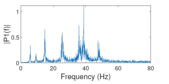
Figure 7: Fourier transform for damage pattern 2: sensor on the right side of the first floor
To identify the instant at which the damage occurred, we decided to use a bandpass filter and perform the frequency-time decomposition using the Hilbert-Huang transform. Fig. 7 shows that the first natural frequency could be between 5 and 10,5 Hz. Therefore, a bandpass filter (bandpass (X,(5 10,5), Fs)) was used, and applied EMD was applied as shown in Fig. 8. The first plot corresponds to the filtered signal, and the others are the IMFs corresponding to the decomposition of the measured signal in the first modal response. By applying the Hilbert-Huang transform to all the IMFs, the frequency-time decomposition of the first modal response was obtained.
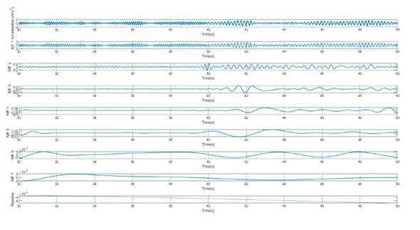
Figure 8: EMD for damage pattern 2 with a bandpass filter: sensor on the right side of the first floor
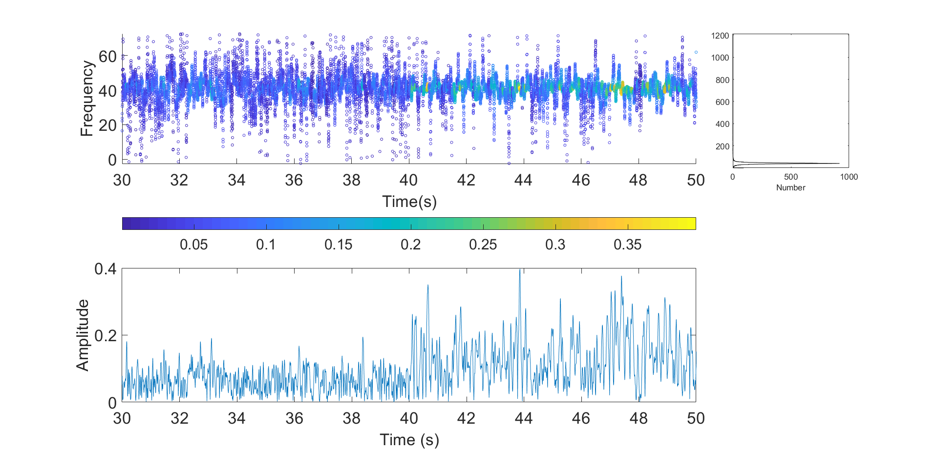
Fig. 9 shows a frequency vs. time plot. The average frequency of the first mode changed from 9,6 to 5,6 Hz at time instant t = 40 s. Therefore, the time instant at which the damage occurred was accurately detected. However, in the other modal responses, the splitting of the natural frequencies was not so prominent. When the Hilbert-Huang transform was applied, the frequency vs. time plots also showed that the change occurred at 40 s.
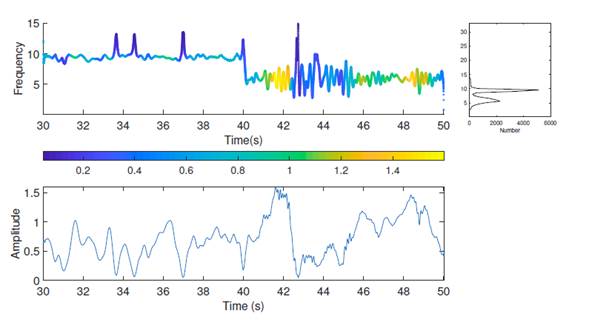
Figure 9: Hilbert-Huang transform for the first modal response (damage pattern 2): sensor on the right side of the first floor
Then, SSA was applied. Fig. 10 presents the RCs of this method. A bandpass filter (bandpass (X,(5 10,5), Fs)) was applied to the signal. Although, in the RC1 and RC2, a change in the signal behavior had already been observed at 40 s, the Hilbert-Huang transform was applied to each RC. Fig. 11 shows the Hilbert-Huang transforms of RC1 for the sensor. The average frequency of the first mode changed from 9,6 to 5,6 Hz at t = 40 s. Therefore, we accurately detected when the damage occurred by using SSA, and the results agreed with those of EMD.
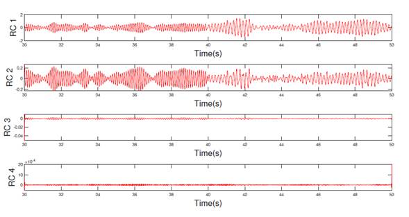
Figure 10: RC for damage pattern 2: sensor on the right side of the first floor
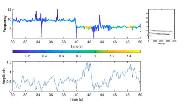
Figure 11: Hilbert-Huang transform for RC1 (damage pattern 2): sensor on the right side of the first floor
Fig. 12 shows the acceleration records of the first and second floors for damage pattern 4. To these signals, a bandpass filter (bandpass(X,(37,5 48), Fs)) was applied, which was obtained from the Fourier transform. Then, the EMD method was used. The first IMFs for each of the floors in Fig. 13 were applied. On all floors, there was a significant change in the behavior of the signal at 40 s. Additionally, the Hilbert-Huang transform was applied, as shown in Fig. 14. Here, the frequency change was small since this damage pattern is considered to be moderate. However, there was a significant change in the amplitude level at 40 s. The accelerations of the other floors showed the same behavior.
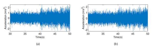
Figure 12: Acceleration records: a) first floor, b) second floor. All plots correspond to damage pattern 4 as obtained from the sensor on the right side in the x-direction.
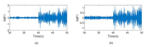
Figure 13: IMF 1: a) first floor, b) second floor. All plots correspond to damage pattern 4, obtained from the sensor on the right side in the x-direction.
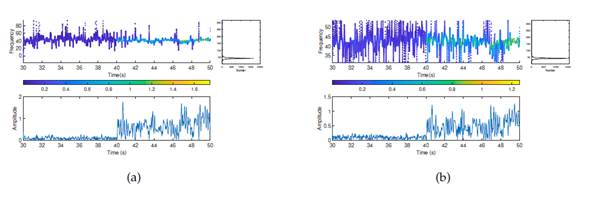
Figure 14: Hilbert-Huang transform for the first modal response: a) first floor, b) second floor. All plots correspond to damage pattern 4.
Then, SSA was applied. Fig. 15 presents the RCs, where, unlike EMD, it is not necessary to apply any filter. Although, in RC1 and RC2, a change in the signal behavior was observed at 40 s, the Hilbert-Huang transform was applied to each RC. Fig. 16 depicts the Hilbert-Huang transforms of RC1 for both sensors. Like EMD, the frequency change was small, but there was a clearly significant change in the amplitude level at 40 s.
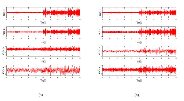
Figure 15: RC for damage pattern 4: (a) first floor, (b) second floor
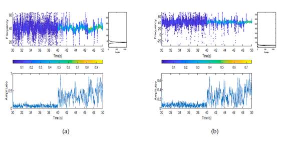
Figure 16: Hilbert-Huang transform for RC1 (damage pattern 4): a) first floor, b) second floor, c) third floor, d) fourth floor
Fig. 17 illustrates the acceleration records of the first and second floors for damage pattern 6. To these signals, a bandpass filter (bandpass (X,(37,5 48), Fs)) was applied, which was obtained from the Fourier transform. Subsequently, the EMD method was used. The first IMF for each of the floors is presented in Fig. 18. Note that the signal changed at 40 s on floors 1 and 4. This was further verified when the Hilbert-Huang transform was applied (Fig. 19), where the frequency change was not so evident on any of the floors. However, on floors 1 and 4, a change in the signal amplitude was observed at 40 s. In contrast, on floors 2 and 3, there was no significant change, which is why it is not necessary to include the graphs. This could indicate that the damage only occurred on floors 1 and 4.
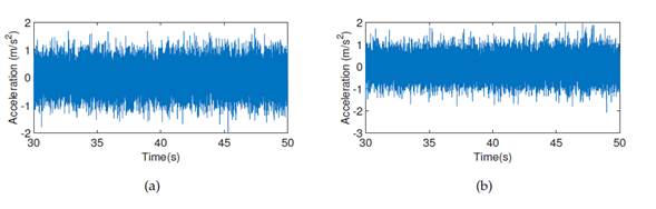
Figure 17: Acceleration records: a) first floor, b) fourth floor. All graphs correspond to damage pattern 6.
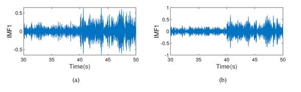
Figure 18: IMF 1: a) first floor, b) fourth floor. All graphs correspond to damage pattern 6.
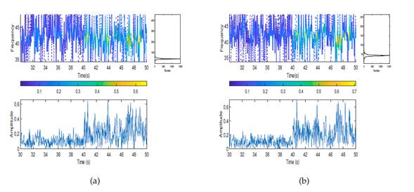
Figure 19: Hilbert-Huang transform for the first modal response: a) first floor, b) fourth floor. All plots correspond to damage pattern 6.
Then, SSA was applied. Fig. 20 presents the RCs. Unlike EMD, it was not necessary to apply any filter. On floors 1 and 4, there was a change in the amplitude of the signal at 40 s, while, on floors 2 and 3, there was no significant change. This could indicate that the damage only occurred on floors 1 and 4, or that the damage on floors 2 and 3 was too slight for the method to detect it. This result can be verified from the amplitude levels shown in the Hilbert-Huang transform (Fig. 21).
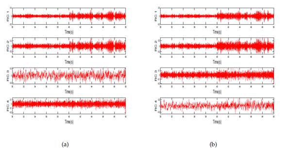
Figure 20: RCs for damage pattern 6: a) first floor, b) fourth floor
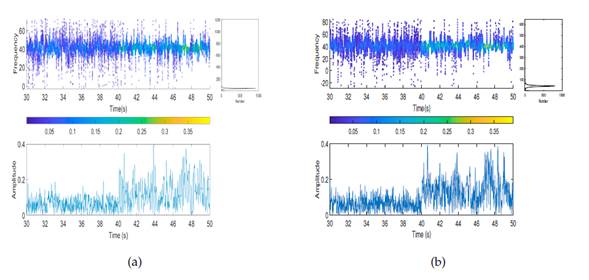
Figure 21: Hilbert-Huang transform for RC1 (damage pattern 6): a) first floor, b) fourth floor
Comparative analysis between EMD and SSA
Based on the above, it can be stated that, when the damage is severe, the characteristic frequency of the signal changes over time, so the empirical distribution of the frequencies is bimodal, which indicates the presence of two characteristic frequencies of the signal, one before and the other after the damage. On the other hand, when there is no damage, the signal retains its fundamental frequency over time.
In order to evaluate the effectiveness of both methods, a Monte Carlo simulation study was conducted, wherein a vibration signal for each type of damage was initially generated. They were like those performed in the previous section, where the noise is normal with a zero mean and one variance. The null hypothesis was that the distribution of frequencies was unimodal, in which case there should be no change in the fundamental frequency of the signal. The alternative hypothesis involved the presence of more than one mode, indicating structural damage. Note that, if the p-value of the statistical test is less than 0,05 (the significance level), the null hypothesis is rejected, and the test detects damage. To control the included random noise and other factors inherent to the simulation, the procedure was repeated 1.000 times. The result of these simulations is the percentage of detection in each damage scenario.
Fig. 22 shows the results of this simulation study, namely the detection percentage for each of the methods.We concluded that, for severe damage, both methods ideally identified the damage However, for damage patterns 3, 4, and 6, the detection capacity of both methods decreased substantially (note that it was evaluated through the identification of frequency changes). This is due to the fact that, for these damage patterns, the frequency variation is 1 Hz or less, as presented in 18. Generally, SSA exhibits better statistics than EMD. It is worth mentioning that the script to apply the hypothesis test was developed in the Python language.
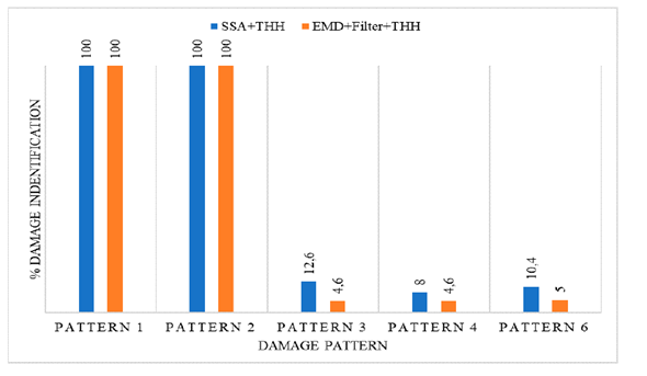
Figure 22: Percentage of damage identification for each method
Conclusions
The EMD method, along with a high pass filter, detected severe damage when the acceleration records had low or no noise.
When the acceleration records were contaminated with noise, the likelihood of EMD detecting the damage decreased dramatically. To reduce the noise phenomenon, the Hilbert-Huang transform was applied. EMD, along with a bandpass filter and the Hilbert-Huang transform allowed detecting severe, moderate, and slight damage with a noise level of 10 %.
The SSA method with high-pass filters detected severe damage when the acceleration records had low or no noise.
When the acceleration records were contaminated with noise and the damage patterns were severe (patterns 1 and 2), SSA, bandpass filters, and the Hilbert-Huang transform could effectively detect the damage.
When the damage was moderate or mild (patterns 3, 4, and 6), SSA detected the damage without any filter, and it was not necessary to apply the Hilbert-Huang transform in any of its components (RCs).
One of the advantages of SSA over EMD is that, for moderate or mild damage patterns, it does not require filters or the use of the Hilbert-Huang transform to detect the damage.
When the damage was severe, both methods showed a noticeable change in the fundamental frequency. However, when the damage was slight, the change in fundamental frequency was not apparent. However, a significant change in the amplitude level was observed. In general, we found that SSA is more effective in detecting damage
References
License
Copyright (c) 2023 González, E. C., Salcedo, G. E., and Cano, L.

This work is licensed under a Creative Commons Attribution-NonCommercial-ShareAlike 4.0 International License.
![]()
From the edition of the V23N3 of year 2018 forward, the Creative Commons License "Attribution-Non-Commercial - No Derivative Works " is changed to the following:
Attribution - Non-Commercial - Share the same: this license allows others to distribute, remix, retouch, and create from your work in a non-commercial way, as long as they give you credit and license their new creations under the same conditions.

2.jpg)