DOI:
https://doi.org/10.14483/23448393.20632Publicado:
2023-10-17Número:
Vol. 28 Núm. 3 (2023): Septiembre-diciembreSección:
Ingeniería Eléctrica, Electrónica y TelecomunicacionesPerformance Analysis of a Backward/Forward Algorithm Adjusted to a Distribution Network with Nonlinear Loads and a Photovoltaic System
Análisis del desempeño de un algoritmo Backward/Forward ajustado a una red de distribución con cargas no lineales y un sistema fotovoltaico
Palabras clave:
Backward/forward, Norton model, nonlinear loads, PV system, Simulink (en).Palabras clave:
backward/forward, modelo Norton, cargas no lineales, sistema FV, Simulink (es).Descargas
Referencias
S. Ouali and A. Cherkaoui, “An improved backward/forward sweep power flow method based on a new network information organization for radial distribution systems,” J. Elect. Comp. Eng., vol. 2020, art. 5643410, 2020. https://doi.org/10.1155/2020/5643410 DOI: https://doi.org/10.1155/2020/5643410
M. Milovanović, J. Radosavljević, and B. Perović, “A backward/forward sweep power flow method for harmonic polluted radial distribution systems with distributed generation units,” Int. Trans. Elect. Energy Syst., vol. 30, no. 5, pp. 1-17, 2020. https://doi.org/10.1002/2050-7038.12310 DOI: https://doi.org/10.1002/2050-7038.12310
A. Garcés-Ruiz, “Flujo de potencia en redes de distribución eléctrica trifásicas no equilibradas utilizando Matlab: Teoría, análisis y simulación cuasi-dinámica,” Ing., vol. 27, no. 3, art. e19252, 2022. https://doi.org/10.14483/23448393.19252 DOI: https://doi.org/10.14483/23448393.19252
A. Suchite-Remolino, H. F. Ruiz-Paredes, and V. Torres-Garcia, “A new approach for PV nodes using an efficient backward/forward sweep power flow technique,” IEEE Latin America Trans., vol. 18, no. 6, pp. 992-999, 2020. https://doi.org/10.1109/TLA.2020.9099675 DOI: https://doi.org/10.1109/TLA.2020.9099675
R. Taheri, A. Khajezadeh, M. H. Rezaeian Koochi, and A. Sharifi Nasab Anari, “Line independency-based network modelling for backward/forward load flow analysis of electrical power distribution systems,” Turkish J. Elect. Eng. Comp. Sci., vol. 27, no. 6, pp. 4551-4566, 2019. https://doi.org/10.3906/elk-1812-137 DOI: https://doi.org/10.3906/elk-1812-137
X. Wang, M. Shahidehpour, C. Jiang, W. Tian, Z. Li, and Y. Yao, “Three-phase distribution power flow calculation for loop-based microgrids,” IEEE Trans. Power Syst., vol. 33, no. 4, pp. 3955-3967, 2018. https://doi.org/10.1109/TPWRS.2017.2788055 DOI: https://doi.org/10.1109/TPWRS.2017.2788055
A. Al-sakkaf and M. AlMuhaini, “Power flow analysis of weakly meshed distribution network including DG,” Eng. Technol. App. Sci. Res., vol. 8, no. 5, pp. 3398-3404, 2018. https://doi.org/10.48084/etasr.2277 DOI: https://doi.org/10.48084/etasr.2277
M. Milovanović, J. Radosavljević, B. Perović, and M. Dragičević, “Power flow in radial distribution systems in the presence of harmonics,” Int. J. Elect. Eng. Comp., vol. 2, no. 1, pp. 10-19, 2019. https://doi.org/10.7251/IJEEC1801011M DOI: https://doi.org/10.7251/IJEEC1801011M
D. Buła and M. Lewandowski, “Steady state simulation of a distributed power supplying system using a simple hybrid time-frequency model,” App. Math. Comp., vol. 319, pp. 195-202, 2018. https://doi.org/10.1016/j.amc.2017.02.028 DOI: https://doi.org/10.1016/j.amc.2017.02.028
M. A. Amini, A. Jalilian, and M. R. Pour Behbahani, “Fast network reconfiguration in harmonic polluted distribution network based on developed backward/forward sweep harmonic load flow,” Elect. Power Syst. Res., vol. 168, pp. 295-304, 2019. https://doi.org/10.1016/j.epsr.2018.12.006 DOI: https://doi.org/10.1016/j.epsr.2018.12.006
J. C. Hernandez, F. J. Ruiz-Rodriguez, F. Jurado, and F. Sanchez-Sutil, “Tracing harmonic distortion and voltage unbalance in secondary radial distribution networks with photovoltaic uncertainties by an iterative multiphase harmonic load flow,” Elect. Power Syst. Res., vol. 185, art. 106342, 2020. https://doi.org/10.1016/j.epsr.2020.106342 DOI: https://doi.org/10.1016/j.epsr.2020.106342
F. J. Ruiz-Rodriguez, J. C. Hernandez, and F. Jurado, “Iterative harmonic load flow by using the point-estimate method and complex affine arithmetic for radial distribution systems with photovoltaic uncertainties,” Int. J. Elect. Power Energy Syst., vol. 118, art. 105765, 2020. https://doi.org/10.1016/j.ijepes.2019.105765 DOI: https://doi.org/10.1016/j.ijepes.2019.105765
A. M. Kettner, L. Reyes-Chamorro, J. K. Maria Becker, Z. Zou, M. Liserre, and M. Paolone, “Harmonic power-flow study of polyphase grids with converter-interfaced distributed energy resources-Part I: Modeling framework and algorithm,” IEEE Trans. Smart Grid, vol. 13, no. 1, pp. 458-469, 2022. https://doi.org/10.1109/TSG.2021.3120108 DOI: https://doi.org/10.1109/TSG.2021.3120108
W. Sun and G. P. Harrison, “Distribution network hosting capacity assessment: Incorporating probabilistic harmonic distortion limits using chance constrained optimal power flow,” IET Smart Grid, vol. 5, no. 2, pp. 63-75, 2022. https://doi.org/10.1049/stg2.12052 DOI: https://doi.org/10.1049/stg2.12052
R. Satish, K. Vaisakh, A. Y. Abdelaziz, and A. El-Shahat, “A novel three-phase harmonic power flow algorithm for unbalanced radial distribution networks with the presence of D-STATCOM devices,” Electronics (Switzerland), vol. 10, no. 21, art. 2663, 2021. https://doi.org/10.3390/electronics10212663 DOI: https://doi.org/10.3390/electronics10212663
R. Satish, P. Kantarao, and K. Vaisakh, “A new algorithm for harmonic impacts with renewable DG and non-linear loads in smart distribution networks,” Technol. Econ. Smart Grids Sust. Energy, vol. 7, no. 1, art. 8, 2022. https://doi.org/10.1007/s40866-022-00134-1 DOI: https://doi.org/10.1007/s40866-022-00134-1
D. Chathurangi, U. Jayatunga, M. Rathnayake, A. Wickramasinghe, A. Agalgaonkar, and S. Perera, “Potential power quality impacts on LV distribution networks with high penetration levels of solar PV,” presented at Int. Conf. Harmon. Qual. Power, ICHQP, Ljubljana, Slovenia, 2018. https://doi.org/10.1109/ICHQP.2018.8378890 DOI: https://doi.org/10.1109/ICHQP.2018.8378890
Z. Deng, G. Todeschini, K. L. Koo, and M. Mulimakwenda, “Modelling renewable energy sources for harmonic assessments in DIgSILENT PowerFactory: Comparison of different approaches,” in 11th Int. Conf. Simul. Mod. Method. Technol. App., SIMULTECH 2021, 2021, pp. 130-140. https://doi.org/10.5220/0010580101300140 DOI: https://doi.org/10.5220/0010580101300140
W. Yuan, X. Yuan, L. Xu, C. Zhang, and X. Ma, “Harmonic loss analysis of low-voltage distribution network integrated with distributed photovoltaic,” Sustainability (Switzerland), vol. 15, no. 5, art. 4334, 2023. https://doi.org/10.3390/su15054334 DOI: https://doi.org/10.3390/su15054334
S. M. Ahsan, H. A. Khan, A. Hussain, S. Tariq, and N. A. Zaffar, “Harmonic analysis of grid-connected solar PV systems with nonlinear household loads in low-voltage distribution networks,” Sustainability (Switzerland), vol. 13, no. 7, art. 3709, 2021. https://doi.org/10.3390/su13073709 DOI: https://doi.org/10.3390/su13073709
G. Osma-Pinto and G. Ordóñez-Plata, “Measuring factors influencing performance of rooftop PV panels in warm tropical climates,” Solar Energy, vol. 185, pp. 112-123, 2019. https://doi.org/10.1016/j.solener.2019.04.053 DOI: https://doi.org/10.1016/j.solener.2019.04.053
G. Osma-Pinto and G. Ordóñez-Plata, “Measuring the effect of forced irrigation on the front surface of PV panels for warm tropical conditions,” Energy Rep., vol. 5, pp. 501-514, 2019. https://doi.org/10.1016/j.egyr.2019.04.010 DOI: https://doi.org/10.1016/j.egyr.2019.04.010
A. Martinez-Penaloza, L. Carrillo-Sandoval, and G. Osma-Pinto, “Determination and performance analysis of the Norton equivalent models for fluorescents and LED recessed lightings,” presented at 2019 IEEE W. Power Elect. Power Qual. App., PEPQA 2019, Manizales, Colombia, 2019. https://doi.org/10.1109/PEPQA.2019.8851554 DOI: https://doi.org/10.1109/PEPQA.2019.8851554
A. Martínez-Peñaloza, L. Carrillo-Sandoval, G. Malagón-Carvajal, C. Duarte-Gualdrón, and G. Osma-Pinto, “Determination of parameters and performance analysis of load models for fluorescent recessed lightings before power supply signal,” DYNA (Colombia), vol. 87, no. 215, pp. 163-173, 2020. https://doi.org/10.15446/dyna.v87n215.85239 DOI: https://doi.org/10.15446/dyna.v87n215.85239
A. Martínez-Peñaloza and G. Osma-Pinto, “Analysis of the performance of the Norton equivalent model of a photovoltaic system under different operating scenarios,” Int. Review Elect. Eng. – IREE, vol. 16, no. 4, pp. 328-343, 2021. https://doi.org/10.15866/iree.v16i4.20278 DOI: https://doi.org/10.15866/iree.v16i4.20278
A. Martínez Peñaloza, G. Osma-Pinto, and G. Ordóñez-Plata, “Parameter determination of coupled and decoupled admittance matrix methods of the Norton equivalent model for an air extractor,” Tecnura, vol. 26, no. 74, pp. 17-34, 2022. https://doi.org/10.14483/22487638.18806 DOI: https://doi.org/10.14483/22487638.18806
Z. Guo et al., “Aggregate harmonic load models of residential customers. Part 2: Frequency-domain models,” in 2019 IEEE PES Innov. Smart Grid Technol. Europe, ISGT-Europe, 2019, pp. 1-5. https://doi.org/10.1109/ISGTEurope.2019.8905746 DOI: https://doi.org/10.1109/ISGTEurope.2019.8905746
X. Xu et al., “Aggregate harmonic fingerprint models of PV inverters. Part 1: Operation at different powers,” in Int. Conf. Harmon. Qual. Power, ICHQP, 2018 pp. 1-6. https://doi.org/10.1109/ICHQP.2018.8378824 DOI: https://doi.org/10.1109/ICHQP.2018.8378824
S. Muller et al., “Aggregate harmonic fingerprint models of PV inverters. Part 2: Operation of parallel-connected units,” in Int. Conf. Harmon. Qual. Power, ICHQP, 2018, pp. 1-6. https://doi.org/10.1109/ICHQP.2018.8378835 DOI: https://doi.org/10.1109/ICHQP.2018.8378835
E. Tavukcu, S. Müller, and J. Meyer, “Assessment of the performance of frequency domain models based on different reference points for linearization,” Renewable Energy Power Qual. J., vol. 17, no. 17, pp. 435-440, 2019. https://doi.org/10.24084/repqj17.337 DOI: https://doi.org/10.24084/repqj17.337
Cómo citar
APA
ACM
ACS
ABNT
Chicago
Harvard
IEEE
MLA
Turabian
Vancouver
Descargar cita
Recibido: 24 de junio de 2023; Revisión recibida: 30 de mayo de 2023; Aceptado: 5 de julio de 2023
Abstract
Context:
The backward/forward (BF) algorithm is a sweep-type technique that has recently been used as a strategy for the power flow analysis of ill-conditioned networks. The purpose of this study is to evaluate the performance of the BFalgorithm compared to that of a computational tool such as Simulink, with both strategies adjusted to the operating conditions of a distribution network with nonlinear components (loads and photovoltaic system), unbalanced loads, and harmonic distortion in the voltage and current signals.
Method:
The study case is a low-voltage distribution network with a radial topology, unbalanced loads, and nonlinear components. The BF algorithm is adjusted to consider two approaches of the Norton model: a coupled admittance matrix and a decoupled admittance matrix. The latter is also used in the network model created in Simulink. The performance of the algorithm is evaluated by analyzing 18 operation scenarios defined according to the presence and use intensity of the loads and solar irradiance levels (low and high).
Results:
In general, the three strategies could successfully determine the waveform and RMS values of the voltage signals with errors of less than 0,8 and 1,3 %, respectively. However, the performance of the strategies for the estimation of current signals and power parameters shows errors of 5-300% depending on the level of solar irradiance at which the photovoltaic system operates.
Conclusions:
The results show that the BF strategy can be used to analyze unbalanced power grids with increasing penetration of renewable generation and the integration of nonlinear devices, but the performance of this strategy depends on the load model applied to represent the behavior of nonlinear devices and generation systems.
Keywords:
backward/forward, Norton model, nonlinear loads, PV system, Simulink.Resumen
Contexto:
El algoritmo backward/forward (BF) es una técnica de barrido que se ha utilizado recientemente como estrategia para el análisis de flujo de energía de redes mal acondicionadas. El objetivo de este estudio es evaluar el desempeño del algoritmo BF comparado con el de una herramienta computacional como Simulink, con ambas estrategias ajustadas a las condiciones de operación de una red de distribución con componentes no lineales (cargas y sistema fotovoltaico), desbalance en las cargas y distorsión armónica en tensión y corriente.
método:
El caso de estudio es una red de distribución de baja tensión con topología radial, cargas desequilibradas y componentes no lineales. El algoritmo BF se ajusta para considerar dos enfoques del modelo Norton: matriz de admitancia acoplada y matriz de admitancia desacoplada. Este ultimo también se utiliza en el modelo de red creado en Simulink. El desempeño del algoritmo se evalúa mediante el análisis de 18 escenarios de funcionamiento definidos según la presencia e intensidad de uso de las cargas y los niveles de irradiancia solar (baja y alta).
Resultados:
En general, las tres estrategias podría determinar con éxito los valores de forma de onda y RMS de las señales de tensión con errores menores de 0,8 y 1,3% respectivamente. Sin embargo, el desempeño de las estrategias para la estimación de señales de corriente y parámetros de potencia presenta errores de 5-300% dependiendo del nivel de irradiancia solar en el cual el sistema fotovoltaico se encuentre operando.
Conclusiones:
Los resultados muestran que la estrategia BF se puede utilizar para analizar redes eléctricas desbalanceadas con creciente penetración de generación renovable e integración de dispositivos no lineales, pero el rendimiento de la misma depende del modelo de carga aplicado para representar el comportamiento de los dispositivos no lineales y de los sistemas de generación.
Palabras clave:
backward/forward, modelo Norton, cargas no lineales, sistema FV, Simulink.Introduction
Power flow analysis is a tool that makes it possible to conduct studies on power generation dispatch,distribution network analysis, load control, network reconfiguration planning, and distributed energy resource (DER) integration (e.g., photovoltaic (PV) generators, electric vehicles, and energy storage units) 1.
However, solving a power flow is a complex task due to the number of variables and their mathematical formulations. Therefore, iterative method have been proposed, such as the Gauss-Seidel approach, impedance matrices, and the backward/forward (BF) technique with admittance summation. These methods are based on a linear system that operates only at the fundamental frequency 2,3.
In recent years, sweep iterative methods such as BF have been used to study radial distribution networks, as they can ensure the convergence of the power flow while considering network characteristics such as load imbalance and the high R/X ratio of conductors 1,4,5.
In addition, sweep methods are a viable option for conducting studies on the behavior of a grid with distributed generation integration and the presence of nonlinear devices 2,6,7.
Moreover, variants of harmonic power flow analysis algorithms have been proposed for application in distribution networks, which consider frequency variations associated with DERs and nonlinear loads. Among these, algorithms in the frequency domain stand out for their effectiveness in reducing computational times 2,8-16.
For example, 10 proposed a method based on harmonic sweeps to improve the accuracy of harmonic analyses in distribution systems. 2 proposed a rapid and effective harmonic sweep method that solves harmonic power flows for radial distribution networks with integrated distributed generation units. 16 presented a new algorithm for fundamental power flow and harmonic power flow, with the aim of evaluating the impacts of integrating renewable generation and nonlinear loads in distribution grids. Kettner et al. 13 proposed a method to solve the three-phase harmonic power Flow with the integration of CIDERs in the systems.
It is considered to be a generic and modular representation of system elements and the coupling between harmonics.
Some researchers have adjusted the BF algorithm to introduce distributed generators and nonlinear loads. 1 proposed a new BF-based power flow analysis approach that organizes grid information to facilitate programming by reducing the search for connections between nodes.
4 presented an alternative approach to the BF sweep, whose advantage is convergence speed in distribution networks with controlled voltage nodes (PV). 5 proposed a method based on the concept of independent lines to consecutively order the distribution network lines, which is subsequently applied to the Kirchhoff law-based BF sweep algorithm.
Although the algorithms for analyzing the power flows of distribution networks propose adaptations to the new conditions, few studies have considered integrating PV generation, load imbalance, and nonlinear loads (single-phase, two-phase, or three-phase) simultaneously.
Additionally, considering nonlinear devices in power flow analysis requires models that represent their harmonic nature and take the harmonic interaction between voltage and current into account 8,13-16. It is common to use the fundamental frequency-dependent current source model for these loads, which does not consider such harmonic interactions 2,8,14-16. In light of this, other load models may be suitable, such as the Norton equivalent coupled admittance matrix model, as well as proposing or studying the performance of harmonic power-flow solution algorithms that consider the actual conditions of distribution networks.
Therefore, studies on distribution networks with these characteristics are necessary; they allow, among other things, characterizing the harmonic distortion pollution caused by the high presence of electronic loads and the increasing penetration of PV systems in low-voltage distribution networks 10, which tend to increase power losses and interference in communications while decreasing the lifetime of the installed equipment 14,17-20.
In this sense, the contribution of this lies in the fact that it determined the performance of a BF sweep-type algorithm whose mathematical approach was adapted to the conditions of the electricity distribution network in a university building (unbalanced loads, nonlinear loads, the integration of a PV system, and harmonic distortion in the feed signal) in order to solve the harmonic power flow. Moreover, the nonlinear devices and PV system were modeled using the coupled and decoupled admittance matrix methods of the Norton equivalent model.
The performance analysis consisted of an evaluation of the strengths and weaknesses of three power flow solution strategies: BF with the coupled Norton model (BF-NC), BF with the decoupled Norton model (BF-ND), and Simulink with the decoupled Norton model (SIM-ND). This evaluation compared the waveform results and RMS values of the voltage and current signals and power parameters, such as apparent, active, non-active power as well as the power factor.
The SIM-ND and BF-ND strategies allowed inferring the effect of adjusting the traditional BF algorithm, given that they employ the same data and input parameters. The BF-NC strategy was studied to determine the implications of using a more complex load model in the mathematical approach of the BF algorithm.
Methodology
Figure 1 illustrates the methodology used in this study, which begins with a description of the case study (Section 2.1) and the modeling of the network components (Section 2.2). Then, it presents the adaptation of the BF algorithm for a three-phase, unbalanced, and nonlinear case study (Section 2.3), along with the network’s modeling in Simulink (Section 2.4), and the definition of simulation scenarios (Section 2.5). Finally, Section 2.6 is dedicated to the resulting data processing and error indicators (Section 2.6).
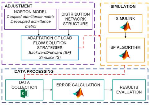
Figure 1: Diagram of the methodology
Study case
The electrical network in the case study is a section belonging to the network of the Electrical Engineering Building of Universidad Industrial de Santander. This building is located in Bucaramanga, Colombia, at 7°8’ North, 73°0’ West. During daylight hours (6 a.m. to 6 p.m.), the temperature ranges between 24 and 28 °C, while the solar irradiance varies between 2,0 and 7,6 kWh/m2 day, with an average of 4,9 kWh/m2 day (21, 22). Fig. 2 presents the solar irradiance of one week for the month of June, 2018. The solar irradiance for that year was used for our case study.
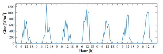
Figure 2: Solar irradiance during a week for the month of June
Fig. 3 shows a five-level building with an area of approximately 2.700 m2. The first four levels are for classrooms and student areas, and the fifth level is for the administrative area. Different strategies for the rational and efficient use of energy (REUE) have been implemented, such as natural lighting and ventilation, green roofs (580 m2), automation systems, and PV generation systems.
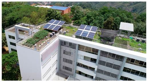
Figure 3: Electrical Engineering Building
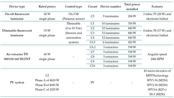
Fig. 4 shows the single-line diagram of the studied network (TP4), with each branch containing lighting loads, air extractors, and THWN 12AWG conductors. There is a TP4 distribution board for the electrical network on the fourth floor of the building. It consists of a lighting sub-board (TALU4) and a common coupling point (PCC) for the PV system installed on the terrace. The TALU4 contains ten single-phase circuits with dimmable luminaires, air extractors (classrooms), and on/off luminaires (bathrooms and corridors). The PV system has the following units: a solar tracker SS-1 (one panel), SFV1 (18 panels), SFV2 (18 panels), and SFV3 (six panels). Table I lists the general characteristics of the luminaires, air extractor, and PV systems.
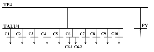
Figure 4: Single-line diagram of the studied low-voltage network
Table I: General characteristics of the loads and PV system
Modeling the elements
The studied distribution network is made up of a transformer, conductors, nonlinear loads, and a PV system. For these components (except for the transformer), it is necessary to establish a dependency on frequency changes in the frequency domain.
The transformer of the building has a capacity of 630 kVA and 13,2 kV/220 V, as well as a Δyn5 connection. This element is defined as the simulated network voltage source and, therefore, as an infinite power node or SLACK with a nominal phase voltage of 127 V.
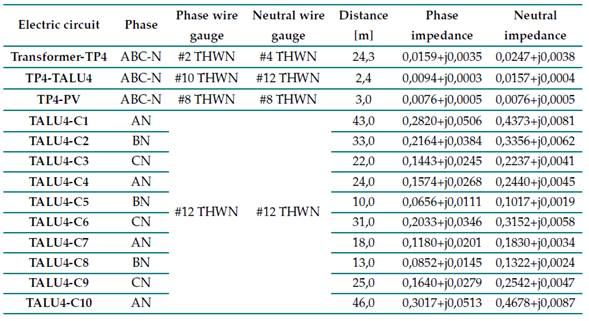
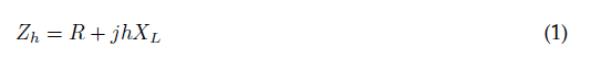
The electrical conductors of the network circuits under study are of the THWN type and of different wire gauges. Their distance corresponds to the separation between the board and load. These elements are represented as frequency-dependent impedance Zh, as expressed in Eq. (1), where h indicates the harmonic order of the frequency under study, R is the resistance, and XL is the inductive reactance. Table II describes the characteristic of the electrical wires of each network circuit.
Table II: Characteristics of the electric wires
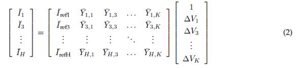
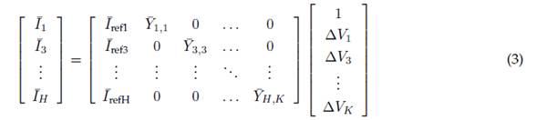
Finally, the nonlinear loads and the PV system are represented by Norton equivalent models of coupled and decoupled admittance matrices, as shown in Eqs. (2) and (3), respectively. This coupled approach allows the study of the harmonic interaction between the voltage and the current signals.
Here,
 represents the current vector of the device,
 frequency concatenated with the
 admittance matrix,
 is the vector of the voltage signal variations. The dimensions of the H and K models indicate the highest odd harmonic order used for the current and voltage signals, respectively.
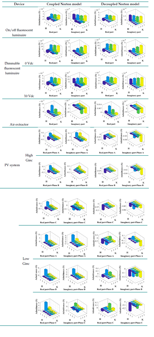
Table III presents the coupled and decoupled Norton models for each nonlinear element (luminaires, extractors, and the PV system). The model for each single-phase load (luminaire or air extractor) was graphically represented by the real and imaginary parts of the admittance matrix for each operating condition. The PV system is a three-phase component, represented by six admittance matrices for each operating condition. The on/off luminaires and extractors have one operating condition, the dimmable luminaires have two operating conditions according to dimmer level (0 and 10 Vdc), and the PV system has three operating conditions according to solar irradiance (high and low) (23-26).
Table III: Norton equivalent models for each element
Adapted backward/forward (BF) iterative algorithm
Generally, the BF iterative sweep algorithm using Kirchhoff’s laws is employed to solve the power flows of distribution networks. It orders the network nodes to systematize the iterative process of calculating the currents that flow through the conductors from the currents injected into the nodes. Similarly, it helps to calculate the voltages in the lower nodes, starting from the voltage of the source node. Fig. 5 illustrates the nodal ordering applied to the scheme.
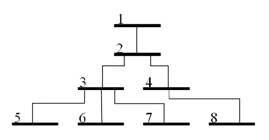
Figure 5: Example of nodal ordering scheme
For this case study, adjusting the algorithm’s mathematical approach to the characteristics of the network allows considering unbalanced loads, harmonic distortion in the feeder, and the use of the Norton model to represent nonlinear loads and the PV system, as shown in Fig. 6.
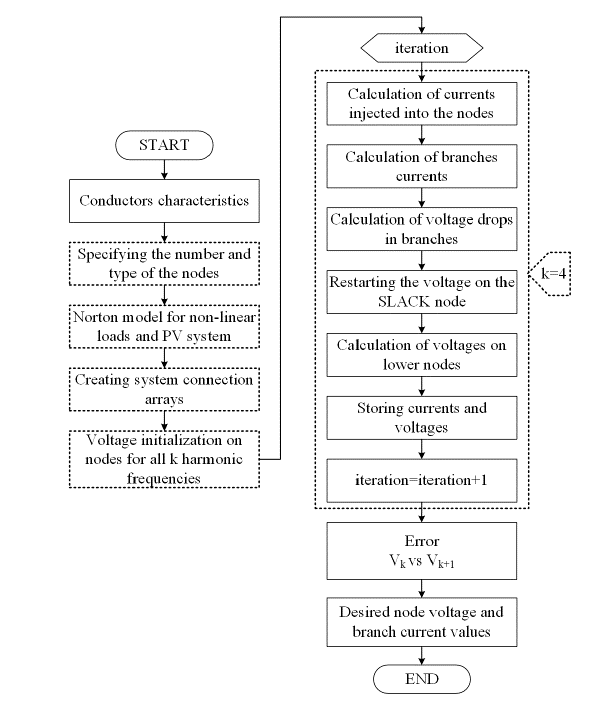
Figure 6: Adapted backward-forward (BF) algorithm flowchart
The dotted blocks in Fig. 6 highlight the process added or adjusted according to network characteristics, such as the input of the Norton models of nonlinear loads and the PV system and the initialization of the voltage signal for all k frequencies. Calculations within the iterative process are consecutively performed for each k frequency. The third, fifth, and seventh harmonic orders were the harmonic frequencies adopted for the study, as they were the most representative within the feeder signal. Therefore, the frequency value of k was 4.
There is a general stage involving the initialization of the conditions for the power flow, which includes the input of the data characteristics of the network, the input of the Norton models for each of the nonlinear loads and the PV system, the creation of arrays that represent the connections of the circuits in the network, and the input of the initial conditions of the voltage signal into each of the nodes of the network. Note that the initial voltage conditions were obtained from a prior review of the voltaje signals of the studied electrical network at different times of the day. In addition, the initial conditions of each node corresponded to the voltage of the SLACK bus.
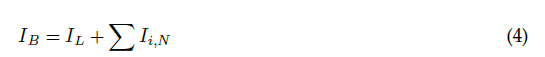
The iterative process of this method consists of two sub-processes. First, the backward sweep calculates the injected currents in the load nodes and PV system according to the Norton model (BF-NC and BF-ND). The current IB flowing through branches is calculated using Eq. (4), where IL is the load or PV system current connected to the node, and Ii,N is the current of the branches i connected to the node N.
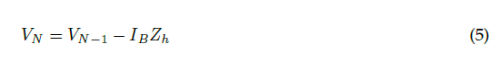
Next, the forward sweep is initialized and calculates the voltage drops of the branches, considering the I B currents and the specific impedances of each conductor. The node voltages were obtained progressively from the SLACK node to the farthest node. At the beginning of each forward sweep cycle, it is necessary to maintain the tension of the SLACK node in its initial conditions and apply Eq. (5), where VN−1 is the voltage of the upper node, VN is the voltage of the lower node, and IBZh represents the voltage drop in the branches.
The node voltage and branch current data are stored in arrays and exported to an Excel file. After finishing the iterative process, the percentage error in magnitude and the absolute error in phase angles between the current and previous iteration data are calculated to find the desired nodal voltage Branch current values.
Modeling the electric network in Simulink
The main objective of this study was to analyze the performance of the BF algorithm adjusted and programmed in MATLAB. To corroborate the results obtained by the BF-ND strategy, the electrical network was modeled in Simulink, considering the use of the decoupled Norton model to represent the loads and the PV system (SIM-ND strategy).
Simulink is a tool that solves power flows using the approach and solution of the state equations of the model in the frequency domain.
The modeling of the studied network considered its characteristics and the most representative odd harmonic orders (third, fifth, and seventh). The network was represented by four subsystems, one at each frequency (Fig. 7). In addition, there is a subsystem containing result export blocks from Simulink to MATLAB in order to facilitate the treatment of the data and compare them with the values estimated by the BF algorithm. The MATLAB Function and Controlled Current Source blocks allow modeling the loads and the PV system in each subsystem by applying only the Norton decoupled matrix model.
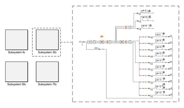
Figure 7: General structure of the Simulink model
Operation scenarios
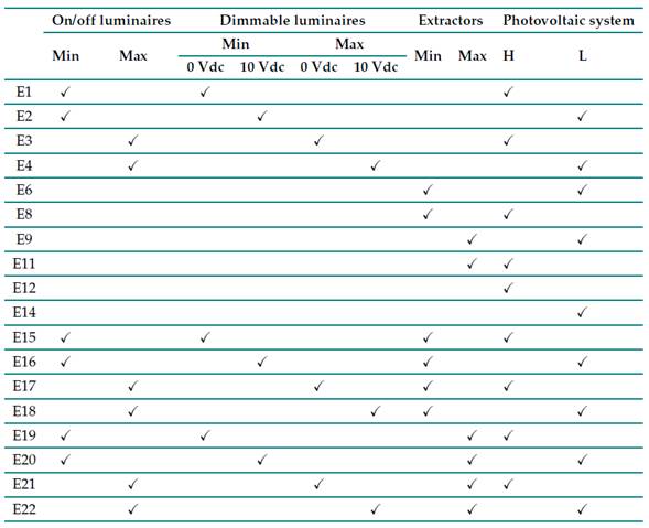
Table IV presents 18 scenarios for the operation of the electricity grid under study, which are based on two inputs. The first input corresponds to the operating conditions of the dimmable luminaires (0 and 10 Vdc), the on/off luminaires, the air extractors (on), and the PV system for two levels of solar irradiance (high-H and low-L). The second input is the representativeness of the number of devices in simultaneous operation.
Table IV: Operation scenarios for the study case
Data processing
At the end of each simulation, the magnitude and phase-angle data of the node voltages, Branch currents, and neutral currents were stored in an Excel file corresponding to each operation scenario. The magnitude and phase angle data were discriminated by each harmonic order under study (fundamental, third, fifth, and seventh).
After the simulation of the operation scenarios had been completed, the normalized root mean square errors (NRMSEs) were calculated by importing the data stored in Excel to the MATLAB Workspace. These errors were estimated from the waveforms obtained using the three analyzed strategies. Similarly, the RMS values of the voltage node and current in the branches were calculated. Finally, the power parameters were estimated to analyze the performance of the strategies in terms of the apparent, active, and non-active power, as well as the power factor.
Results
This section presents the results obtained while estimating the electrical grid voltage, current signals, and power parameters. First, it shows the evolution of method performance (Section 3.1). Then, it presents the analysis of RMS values (Section 3.2), waveforms and NRMSEs (Section 3.3), influence factors (Section 3.4), and network power parameters (S, P, QF, and fp) (Section 3.5). Finally, it presents a brief analysis of the performance of the studied power flow strategies (Section 3.6).
Evolution of the performance of strategies
Fig. 8 shows the evolution of RMS errors in voltage for node TP4 (VTP4) and the current for Branch SLACK-TP4 (ISLACK-TP4), considering the operation scenarios. These errors were calculated for each scenario by selecting average values for each iteration. The results obtained by the BF-ND and BF-NC strategies are acceptable at the end of the second iteration, with average errors of 2,5e5% for the voltaje and 2,0e-2% for the current.
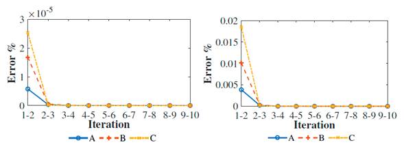
Figure 8: Evolution of the estimation error of the RMS voltage and current values at each iteration
RMS values
Fig. 9 shows the single-line scheme of the studied electrical network that relates the RMS values of nodal voltage and branch current obtained by applying the BF algorithm with decoupled Norton modeling (Fig. 9a) and coupled Norton modeling (Fig. 9b). Specifically, it shows the results for the estimates of Scenario 22, where all the luminaires and air extractors work and the PV system operates under low solar irradiance, which implies high levels of THDi 25.
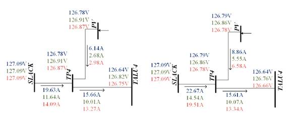
Figure 9: Voltages and currents for operation scenario 22. The blue, green, and red values refer to voltaje or current values for phases A, B, and C, respectively
There was a difference in the VRMS voltage drop values between the lower and SLACK nodes. The two strategies exhibit a similarity of VRMS values, with differences of less than 0,1 V in most load circuits and TP4 and TALU4 nodes.
In terms of the IRMS, there is a significant difference between the values of the two strategies because the coupled model correctly estimates the actual waveform of the current consumed by the load, unlike the decoupled model 23,24,26. This difference is more noticeable in the PV system IRMS injected with differences of 2,7-3,6 A due to the low satisfaction in the estimation of currents by the decoupled model for low solar irradiance 25.
Figs. 10 to 13 show the errors of the RMS values calculated for the three strategies. Fig. 10 shows that the VRMS errors in the TP4 node do not exceed 0,08% in scenarios where the PV system operates at low solar irradiance (e.g., E2, E4, E6, and E9). In comparison, the errors are less than 0,02% for scenarios in which the PV system operates at a high solar irradiance level (e.g., E1, E3, E4, and E7).
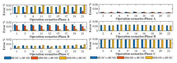
Figure 10: Voltage signal RMS value errors in node TP4 for the operation scenarios
In contrast, Figs. 11 to 13 show the estimation errors regarding the IRMS. Fig. 11 compares the performance of IRMS error strategies for the SLACK-TP4 branch in scenarios where the PV system operates at low solar irradiance levels (E2, E4, E6, E9, E14, E16, E18, E20, and E22). The resulting errors are between 20 and 150 %. These differences between the strategies are caused by the power signal estimation capability of the Norton decoupled model (ND) compared to the Norton coupled model (NC), the latter being the most successful.
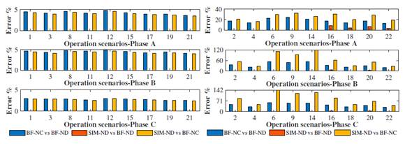
Figure 11: SLACK-TP4 branch current signal RMS values errors for operation scenarios
This may be a consequence of that observed in Fig. 12, where the errors of the IRMS injected by the PV system in scenarios where it operates at low solar irradiance are greater than 20 %. However, in the specific scenarios E16, E18, E20, and E22, phase B and phase C errors exceed 150% when comparing SIM-ND strategies against BF-NC.
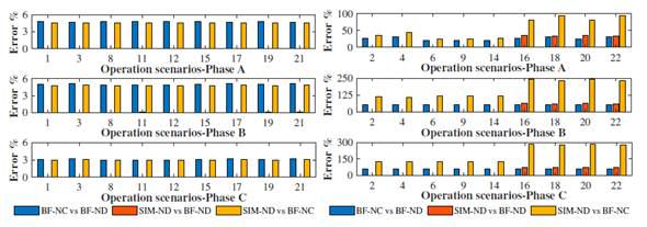
Figure 12: TP4-PV system branch current signal RMS value errors for the operation scenarios
Fig. 13 shows IRMS errors greater than 1,0% in scenarios E1, E3, E15, E17, and E21, where the dimmable luminaires operate with the lowest dimmer level (0 Vdc), which provides greater harmonic distortion (THDi >18 %) than other levels of control (THDi <15 %) (23, 24).
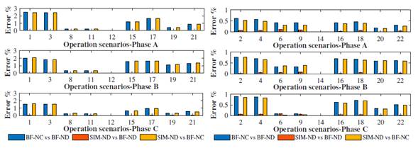
Figure 13: TP4-TALU4 branch current signal RMS value errors for operation scenarios
Waveforms and normalised root mean square errors (NRMSEs)
Fig. 14 presents the characteristics of the waveform of the SLACK bar and those estimated using the three strategies (SIM-ND, BF-ND, and BF-NC). There is a predominance of the flat-top waveform type in these waveforms, where the fifth harmonic order prevails over the third and seventh orders. Similarly, the voltage waveforms obtained using the three strategies are significantly similar. Fig. 15 shows a comparison of the NRMSEs of the voltage signals obtained via the three strategies for the TP4 node in each operation scenario. In general, the values were less than 0,05 %. However, in scenarios where the PV system injects power at a low solar irradiance level and the dimmable luminaires operate at their maximum dimmer level (10 Vdc - E14, E16, E20, and E22), phase A errors are between 0,05 and 0,1% when comparing SIM waveforms-ND with BF-NC, and BF-NC with BF-ND.
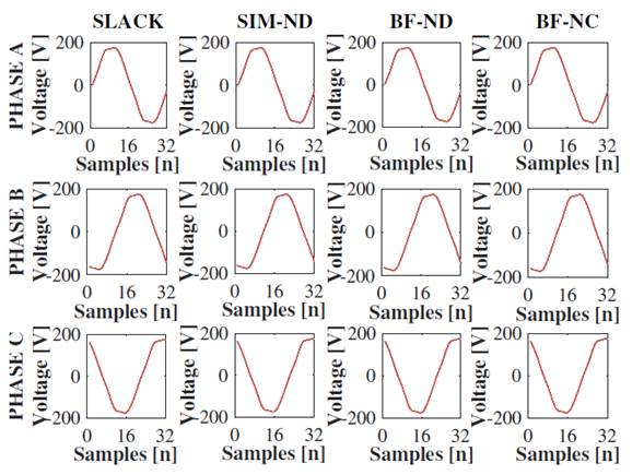
Figure 14: Voltage signal waveforms for all operation scenarios
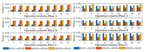
Figure 15: Voltage normalized root mean square errors (NRMSEs) at node TP4 for all operation scenarios
This is the result of an overload in phase A luminaire circuits and the PV system. Similarly, the estimation of the current signal injected by the PV system with the coupled and decoupled Norton models shows differences when analyzing low solar irradiance levels. 25 found that the coupled model estimates the waveform with an NRMSE of less than 2 %, in contrast to the decoupled model, with an error close to 20 %. It should be noted that, although there is prior knowledge of the current performance of Norton models in the modeling of loads and PV systems, this study aims to review the possible impacts of using these models on the voltage and power parameters.
The waveforms of the current signals (Figs. 16, 17, and 18) reveal the differences between the current signals estimated using each of the three strategies.
Fig. 16 clearly shows the differences between the waveforms of the current signals in the SLACK-TP4 branch, considering scenarios where the PV system operates at high solar irradiance (Fig. 16a) and scenarios with low solar irradiance levels (Fig. 16b). The reason for this is the impossibility of the decoupled Norton model to estimate the current signal successfully at this PV system operation level.
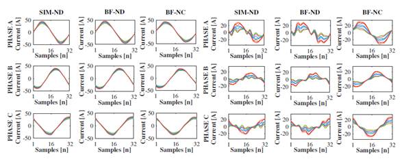
Figure 16: Current signal waveforms on the SLACK-TP4 branch for all operation scenarios
Fig. 17 shows the current waveforms of the TP4-TALU4 branch, where the signals estimated by the three strategies are very similar. However, in the high solar irradiance scenarios (Fig. 17a), the máximum peak current value is 10 A. In the low-solar-irradiance scenarios (Figure 17b), the peak value is 20 A. This is because of the close relationship between the dimmer levels of the dimmable luminaires and the operation of the PV system.
Confirming what is shown in Fig. 16, Fig. 18 reveals the differences between the waveforms of the currents injected by the PV system operating at the two levels of solar irradiance: high (Fig. 18a) and low (Fig. 18b), demonstrating the inability of the decoupled Norton model to estimate the injected current signal at low solar irradiance.
In general, the current waveform injected by the PV system at high solar irradiance levels (Fig. 18a) predominantly affects the current of the SLACK-TP4 branch above the current waveforms from the TALU4 board (Fig. 18a). In contrast, in scenarios with low solar irradiance, the waveform of the current from the TALU4 board (Fig. 18b) is predominant in the SLACK-TP4 branch current above the PV system waveform (Fig. 18b) because the luminaires and air extractors operate at their máximum power, whereas the PV system does not.
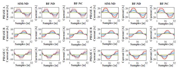
Figure 17: Current signal waveforms on the SLACK-TP4 branch for all operation scenarios
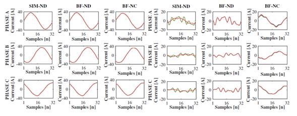
Figure 18: Current signal waveforms on the SLACK-TP4 branch for all operation scenarios
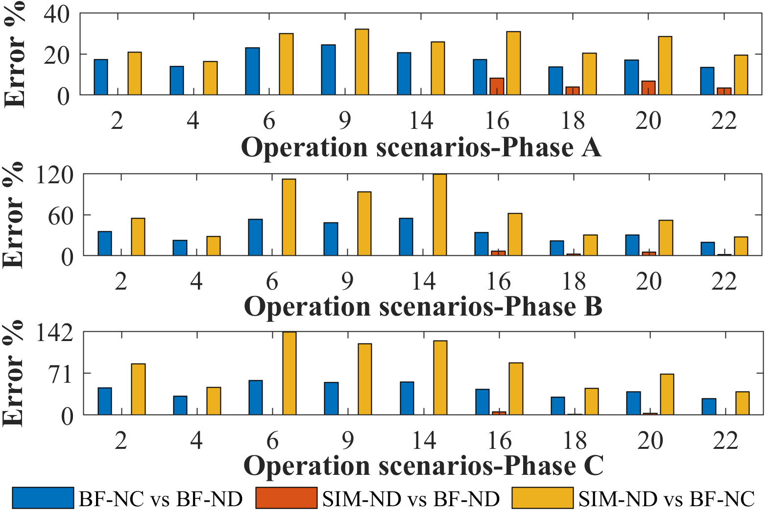
Figs. 19and 20 present the NRMSEs of the waveforms of the current signals in the TP4-PV and TP4-TALU4 branches. Fig. 19 shows the scenarios where the low solar irradiance levels (E2, E4, E6, E9, E14, E16, E18, E20, and E22) work; there is a difference between the waveforms estimated by BF-NC and those estimated by SIM-ND and BF-ND, obtaining NRMSEs greater than 20 %.
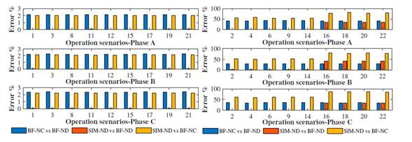
Figure 19: Current NRMSEs in the TP4-PV branch for all operation scenarios
In contrast, in scenarios E1, E3, E7, E8, E15, and E17, the NRMSEs for the estimated current signals were less than 1,0% since the PV system operated at a high irradiance level.
Fig. 20 shows the NRMSEs of the current waveforms of the TP4-TALU4 branch. The NRMSEs obtained are greater than 3,9% for the scenarios where the dimmable luminaire operates at a low dimmer level (0 Vdc - E1, E3, E15, E17, E19, and E21), contrary to the scenarios in which the luminaire operates at a high dimmer level (10 Vdc - E2, E4, E16, E18, E20, and E22), with NRMSEs of less tan 3,3 %.
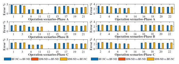
Figure 20: Current NRMSEs in the TP4-TALU4 branch for all operation scenarios
The reason for these errors is that the dimmable luminaires, at the low dimmer level (0 Vdc), have a THDi index higher than 19 %, and, at a high dimmer level (10 Vdc), the THDi index is less than 13% 24.
Factors of influence
The results of the waveform errors of the current signals allow analyzing the potential impact of operating the extractors (minimum and maximum use) and the luminaires (minimum and máximum use and high 10 Vdc dimmer level) in scenarios where the PV system operates at low solar irradiance (E2, E4, E6, E9, E14, E16, E18, E20, and E22). Fig. 21 presents the matrix representations of the impact on the waveform of the current signal of the TP4-PV and TP4-TALU4 branches of the network under study.
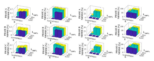
Figure 21: NRMSE load influence matrix for the TP4-TALU4 branch
According to Figs. 21a and 21b, the number of luminaires or air extractors does not influence the waveform errors of the current signals of the branch feeding the TALU4 sub-lighting board. Similarly, NRMSEs close to 3,0 and 4,0% indicate the impact of using the coupled Norton model to represent the luminaires and air extractors, respectively.
Figs. 21c and 21d allow stating that the presence of the luminaires and air extractors does not affect the waveform of the current signal of the PV system, confirming that this estimation depends on the load model used. In this regard, the coupled Norton model more accurately estimates the current signal of the PV system when operating at low solar irradiance levels 25.
Analysis of the power parameters
Considering the results obtained for the waveforms in Section 3.3, an analysis of the power parameters (apparent power, active power, non-active power, and power factor) was performed for all the operation scenarios. Similarly, the errors in these parameters were calculated from the results of the BF-NC strategy.
Fig. 22 shows the power parameter values of the main network branches (SLACK-TP4, TP4-TALU4, and TP4-PV) for scenario 21. This figure reveals the imbalance between the phases of the PV system and the load circuits. In addition, the power factor has values below 0,97 due to the capacitive nature of the loads, which produces an increase in non-active power. It should be noted that the differences in the apparent and active power values and, consequently, in the non-active power values are due to the coupled and decoupled Norton models’ estimation capacity regarding the current signals.
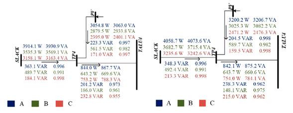
Figure 22: Estimated power parameters for scenario 21
As for the errors in the estimated power parameters when comparing the two BF strategies, Fig. 23 shows the relationship between these variables.
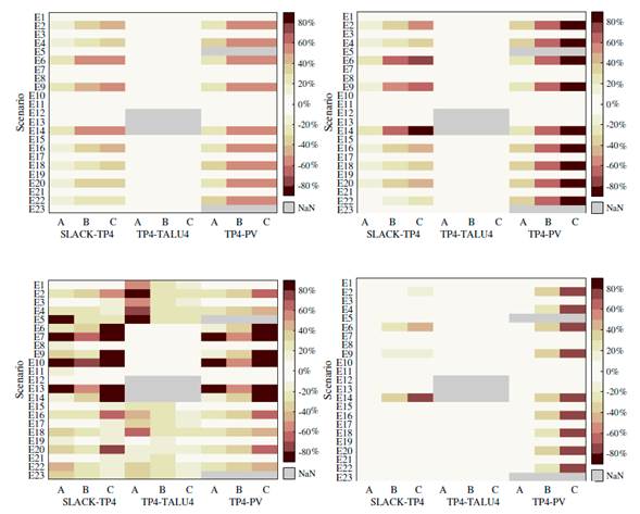
Figure 23: Percentage errors of power parameters (BF-NC vs BF-ND)
Fig. 23a presents the apparent power errors for all the operation scenarios. The errors for the TP4-TALU4 branch are higher than 0,7% in the scenarios where the dimmable luminaire works at its low dimmer level (0 Vdc), contrary to those where the luminaire works at maximum dimmer level (10 Vdc), where the errors are less than 0,8 %. Similarly, the errors in scenarios where the PV system operates at low solar irradiance are above 20 %. In comparison, the errors do not exceed 5% at high solar irradiance.
Fig. 23b presents the errors regarding active power. For the TALU4 lighting sub-board, values between 0,1 and 0,4% can be observed in all operation scenarios. However, the active power errors in the branch from the feeder to the general floor panel (SLACK-TP4) are influenced by the active power errors injected by the PV system. Low solar irradiance scenario errors are between 20 and 90 %, which is reflected in the SLACK-TP4 branch errors, mainly when the PV system works with air extractors.
For the non-active power errors in Fig. 23c, the values are higher than 10% in scenarios where the dimmable luminaires operate at a low dimmer level (0 Vdc). These errors are in the order of 60 and 80 %, respectively, when operating at a high dimmer level (10 Vdc). In addition, the PV system operating at low solar irradiance affects the non-active power errors of the feeder branch (SLACK-TP4).
Following the non-active power errors, the same behavior can be observed for the power factor errors of the TP4-PV branch. Therefore, the error values of the feeder branch to the main floor panel (TP4) are between 30 and 90% for these drivers.
Performance analysis of the strategies
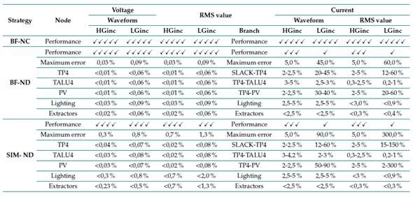
Tables V and VI present a summary of the performance analysis of the studied strategies in terms of the waveforms and RMS values of the voltage, current, and power parameters. The following symbol conventions is used in the Tables, ✓: poor (Error >10), ✓✓: ordinary (6 <Error <10), ✓✓✓: acceptable (1 <Error <5), ✓✓✓✓: good (0,1 <Error <0,9), and ✓✓✓✓✓: excellent (Error <0,1).
The BF-NC strategy was established as a reference for the performance analysis because, within the load models in the frequency domain studied in this research, the Norton model equivalent to the coupled admittance matrix presented in the literature accurately estimates the current of a nonlinear load 23,25,27-30.
According to the results in Table V, the three strategies used exhibit excellent performance (0,03-1,3 %) in estimating the waveforms and RMS values of the voltage signals of the nodes of the electrical network. In terms of current, Table V shows the excellent performance of the BF-NC strategy, as the harmonic interaction is considered in the modeling of the PV system and the loads. However, the BF-ND and SIM-ND strategies, when compared against BF-NC, showed an acceptable performance (5,0 %) in scenarios of high solar irradiance, as well as a poor performance (>10 %) in scenarios of low solar irradiance.
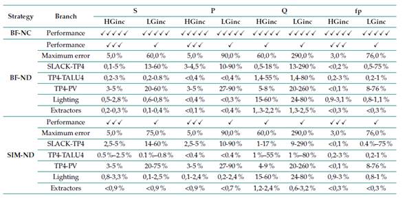
Similarly, Table VI shows the performance analysis of the apparent power (S), active power (P), non-active power (Q), and power factor (fp) parameters. The performance of the BF-ND and SIM-ND strategies regarding non-active power for high and low solar irradiance scenarios is poor (>10 %) because of the behavior of dimmable luminaires working together at the lowest dimmer level (0 Vdc) and the operation of the PV system at low solar irradiance levels.
Note: ✓- Poor, ✓✓- Ordinary, ✓✓✓- Acceptable, ✓✓✓✓- Good, ✓✓✓✓✓- Excellent.
Table V: Performance of the studied strategies in terms of waveforms and RMS voltage values
Note: ✓- Poor, ✓✓- Ordinary, ✓✓✓- Acceptable, ✓✓✓✓- Good, ✓✓✓✓✓- Excellent.
Table VI: Analysis of performance of strategies in terms of power parameters
Conclusions
In this study, the performance of three power flow solution strategies based on the BF sweep iterative method was evaluated while considering nonlinearity and load imbalance, harmonic distortion in the feed signal, and the power injection of the PV system. A detailed analysis of the model’s impact on the voltage and current signals and power parameters was conducted, as the selection of the load model influenced the results of the estimation of these variables.
The NRMSEs were less than 0,8% in terms of voltage when comparing the SIM-ND and BF-ND approaches to BF-NC. Additionally, the maximum error obtained in the estimation of the RMS voltaje values was 1,3 %. Therefore, all three approaches exhibit a satisfactory performance in estimating the voltage signal of the network.
Considering the current results, the NRMSEs and RMS values were less than 5,0% in the operation scenarios where the PV system operated at high solar irradiance levels. In contrast, maximum NRMSEs of 45% (BF-ND) and 90% (SIM-ND) and maximum RMS current errors of 60% (BF-ND) and 300% (SIM-ND) were obtained when the PV system operated at low solar irradiance levels. Therefore, the BF-ND and SIM-ND strategies exhibit an acceptable performance during high solar irradiance operation, in contrast to the values reported for low solar irradiance operation, where the performance was regarded as ordinary.
Meanwhile, regarding the analysis of power parameters, the maximum errors for the apparent power, active power, and power factor were less than 5% in the scenarios of high solar irradiance. The maximum errors were greater than 60% when scenarios of low solar irradiance were analyzed. However, for the non-active power reported by the BF-ND, SIM-ND, and BF-NC approaches, there are errors of 60% for high solar irradiance scenarios and 290% for low solar irradiance scenarios. Therefore, the overall performance obtained by the three approaches in the analysis of power parameters is ordinary.
Finally, the BF algorithm, adjusted to the conditions of the studied distribution network, can easily be applied to other electrical networks with similar nonlinear elements and characteristics. There is also the possibility of integrating other DER types into the network analysis, such as electric vehicles or storage systems
Acknowledgements
Acknowledgments
The authors wish to thank the Department of Electrical, Electronics, and Telecommunications Engineering and the Vice-Principalship for Research and Extension of Universidad Industrial de Santander (Project 2830).
References
Licencia
Derechos de autor 2023 Alejandra Martinez-Peñaloza, Gabriel Ordóñez-Plata, German Alfonso Osma-Pinto

Esta obra está bajo una licencia internacional Creative Commons Atribución-NoComercial-CompartirIgual 4.0.
![]()
A partir de la edición del V23N3 del año 2018 hacia adelante, se cambia la Licencia Creative Commons “Atribución—No Comercial – Sin Obra Derivada” a la siguiente:
Atribución - No Comercial – Compartir igual: esta licencia permite a otros distribuir, remezclar, retocar, y crear a partir de tu obra de modo no comercial, siempre y cuando te den crédito y licencien sus nuevas creaciones bajo las mismas condiciones.

2.jpg)