DOI:
https://doi.org/10.14483/23448393.17589Publicado:
2022-01-04Número:
Vol. 26 Núm. 3 (2021): Septiembre - DiciembreSección:
Ingeniería Eléctrica y ElectrónicaAir Quality Measurement Using an IoT Network: a Case Study
Medición de la calidad del aire mediante una red IoT: un estudio de caso
Palabras clave:
polluting factors, modeling, Kriging method, air quality, area, population (en).Palabras clave:
factores contaminantes, modelación, método de Kriging, calidad del aire, área, población (es).Descargas
Referencias
“Informe anual de Calidad del Aire. Red de monitoreo de la calidad del aire en Bogotá”, Secretaría del Medio Ambiente, 2019. http://rmcab.ambientebogota.gov.co/Pagesfiles/IA%20200531% 20Informe%20Anual%20de%20Calidad%20del%20Aire%20A%C3%B1o%202019.pdf (accessed January 26 th , 2019).
C. H. Cheng and C. C. Ho, “Implementation of multi-channel technology in ZigBee wireless sensor networks”, Comp. Elec. Eng., vol. 56, pp. 498-508, 2016. https://doi.org/10.1016/j.compeleceng.2015.10.002 DOI: https://doi.org/10.1016/j.compeleceng.2015.10.002
N. C. Batista, R. Melicio, V. M. F. Mendes, and J. Figueiredo, “Wireless Monitoring of Urban Wind Turbines by ZigBee Protocol: Support Application Software and Sensor Modules”, Procedia Tech., vol. 17, pp. 461-470, 2014. https://doi.org/10.1016/j.protcy.2014.10.182 DOI: https://doi.org/10.1016/j.protcy.2014.10.182
N. Samotaev, A. Ivanova, K. Oblov, S. Soloviev, and A. Vasiliev, “Wi-fi wireless digital sensor matrix for environmental gas monitoring”, Procedia Tech., vol. 87, pp. 1294-1297, 2014. https://doi.org/10.1016/j.proeng.2014.11.684 DOI: https://doi.org/10.1016/j.proeng.2014.11.684
S. Choudhury, P. Kuchhal, R. Singh, and A. Gehlot, “Zigbee and bluetooth network based sensory data acquisition system”, Procedia Comp. Sc., vol. 48, pp. 367-372, 2015. https://doi.org/10.1016/j.procs.2015.04.195 DOI: https://doi.org/10.1016/j.procs.2015.04.195
J. Gutiérrez, J. F. Villa-Medina, A. Nieto-Garibay, and M. Á. Porta-Gándara, “Automated Irrigation System Using a Wireless Sensor Network and GPRS Module”, IEEE Trans. Inst. Meas., vol. 63, no. 1, pp. 166-176, 2014. https://doi.org/10.1109/TIM.2013.2276487 DOI: https://doi.org/10.1109/TIM.2013.2276487
M. Benghanem, “RETRACTED: A low-cost wireless data acquisition system for weather station monitoring”, Renewable Energy, vol. 35, no. 4, pp. 862-872, 2010. https://doi.org/10.1016/j.renene.2009.08.024 DOI: https://doi.org/10.1016/j.renene.2009.08.024
M. Haefke, S. C. Mukhopadhyay, and H. Ewald, “A Zigbee based smart sensing platform for monitoring environmental parameters,” in 2011 IEEE Int. Inst. Meas. Tech. Conf., Hangzhou, China, Jul. 2011. https://doi.org/10.1109/IMTC.2011.5944154 DOI: https://doi.org/10.1109/IMTC.2011.5944154
A. Marini, P. Mariani, A. Garinei, S. Proietti, P. Sdringola, M. Proietti, and M. Marconi. ”Design of an Urban Monitoring System for Air Quality in Smart Cities”, Smartgreens, pp. 94-101, 2021. https://doi.org/10.5220/0010405200940101 DOI: https://doi.org/10.5220/0010405200940101
Y. Irawan, R. Wahyuni, H. Fonda, M. Hamzah, and R, Muzawi. ”Real Time System Monitoring and AnalysisBased Internet of Things (IoT) Technology in Measuring Outdoor Air”, Int. J. Interac. Mob. Tech., vol. 15, no. 10, 2.021. doi: https://doi.org/10.3991/ijim.v15i10.20707 DOI: https://doi.org/10.3991/ijim.v15i10.20707
N. Bansod and U. Hore, “IoT Based Air Quality Monitoring System”, Int. J. Adv. Res. Sc. Comm. Tech., vol. 6, no. 2, 20707, 2021. https://doi.org/10.48175/IJARSCT-1536 DOI: https://doi.org/10.48175/IJARSCT-1536
A. Nagah and M. Rebaudengo, “LoRaWAN for Air Quality Monitoring System.”, M.Sc. thesis, Politecnico di Torino, Italy, 2021. [Online]. Available: http://webthesis.biblio.polito.it/id/eprint/18045
E. Twahirwa, K. Mtonga, D. Ngabo, and S. Kumaran, “A LoRa enabled IoT-based Air Quality Monitoring System for Smart City", 2021 IEEE World AI IoT Cong. (AIIoT), pp. 0379-0385, 2021. https://doi.org/10.1109/AIIoT52608.2021.9454232 DOI: https://doi.org/10.1109/AIIoT52608.2021.9454232
A. Szpiro, P. D. Sampson, L. Sheppard, and T. Lumley, “Predicting intra-urban variation in air pollution concentrations with complex spatio-temporal dependencies”, Environmetrics, vol. 21, no. 6, pp. 606-631, 2009. https://doi.org/10.1002/env.1014 DOI: https://doi.org/10.1002/env.1014
A. J. Wixted, P. Kinnaird, H. Larijani, A. Tait, A. Ahmadinia, and N. Strachan, “Evaluation of LoRa and LoRaWAN for wireless sensor networks”, in 2016 IEEE SENSORS, Orlando, FL, USA, 2016. https://doi.org/10.1109/ICSENS.2016.7808712 DOI: https://doi.org/10.1109/ICSENS.2016.7808712
M. I. Muzammir, H. Z. Abidin, S. A. C. Abdullah, and F. H. K. Zaman, “Performance Analysis of LoRaWAN for Indoor Application”, 2019 IEEE 9th Symp. Comp. App. Ind. Elec. (ISCAIE), pp. 156-159, 2019. https://doi.org/10.1109/ISCAIE.2019.8743982 DOI: https://doi.org/10.1109/ISCAIE.2019.8743982
A. Lavric and AI Petrariu, "Protocolo de comunicación LoRaWAN: La nueva era de IoT", Conferencia Internacional sobre Desarrollo y Sistemas de Aplicación (DAS), 2018, pp. 74-77. https://doi.org/10.1109/DAAS.2018.8396074 DOI: https://doi.org/10.1109/DAAS.2018.8396074
M. A. Oliver and R. Webster, “Kriging: a method of interpolation for geographical information systems”, Int. J. Geog. Inf. Sys., vol. 4, no. 3, pp. 313-332, 1990. https://doi.org/10.1080/02693799008941549 DOI: https://doi.org/10.1080/02693799008941549
Y. Tong, Y. Yu, X. Hu, and L. He, Análisis del rendimiento de diferentes métodos de interpolación de kriging basados en el índice de calidad del aire en Wuhan", Sexta Conferencia Internacional sobre Control Inteligente y Procesamiento de la Información (ICICIP), pp. 331-335, 2015. https://doi.org/10.1109/ICICIP.2015.7388192 DOI: https://doi.org/10.1109/ICICIP.2015.7388192
R. Hernández-Sampieri, C. Fernández-Collado, and M. P. Baptista-Lucio, Metodología de la Investigación, Ciudad de México, México: McGraw Hill, 2013.
“Mq136 Semiconductor Sensor for Sulfur Dioxide,” Hanwei Electronics Co, 2020. http://www.datasheet.es/download.php?id=904647
"Technical Data Mq-7 Gas Sensor,” Hanwei Electronics Co. https://www.sparkfun.com/datasheets/Sensors/Biometric/MQ-7.pdf (accessed April 17th, 2019).
C.-T. Yang, S.-T. Chen, J.-C Liu, P.-L. Sun, and N. Y. Yen, “On construction of the air pollution monitoring service with a hybrid database converter”, Soft. Comput., vol. 24, pp. 7955-7975, 2020. https://doi.org/10.1007/s00500-019-04079-z DOI: https://doi.org/10.1007/s00500-019-04079-z
“The Sustainable Development Goals Report”, United Nations, 2017. https://unstats.un.org/sdgs/files/report/2017/thesustainabledevelopmentgoalsreport2017.pdf (accessed Jun. 27th, 2019)
R. Li, Z. Li, W. Gao, W. Ding, Q. Xu, and X. Song, “Diurnal, seasonal, and spatial variation of PM2,5 in Beijing”, Sc. Bull., vol. 60, no. 3, pp. 387-395, 2015. https://doi.org/10.1007/s11434-014-0607-9 DOI: https://doi.org/10.1007/s11434-014-0607-9
“Red de Monitoreo de Calidad del Aire de Bogotá,” RMCAB, Secretaria Distrital de Ambiente. http://201.245.192.252:81/home/map (accessed November 13th, 2019).
Cómo citar
APA
ACM
ACS
ABNT
Chicago
Harvard
IEEE
MLA
Turabian
Vancouver
Descargar cita
Recibido: 12 de febrero de 2021; Revisión recibida: 3 de agosto de 2021; Aceptado: 27 de agosto de 2021
Abstract
Context:
The evaluation of air quality in Colombia is localized; it does not go beyond determining whether the level of the polluting gas at a specific point of the monitoring network has exceeded a threshold, according to a norm or standard, in order to trigger an alarm. It is not committed to objectives as important as the real-time identification of the dispersion dynamics of polluting gases in an area, or the prediction of the newly affected population. From this perspective, the presence of polluting gases was evaluated on the university campus of Escuela Colombiana de Ingeniería Julio Garavito, located north of the city of Bogotá, and the affected population was estimated for the month of October, 2019, using the Kriging geostatistical technique.
Method:
This study is part of the design and construction of an auxiliary mobile station that monitors and reports complementary information (CO and SO2 gases) to that provided by the Guaymaral meteorological station, located in the north of Bogotá. This information is transmitted through an IoT network to a server, where a database is created which stores the information on polluting gases reported by the 14 stations of the Bogotá air quality monitoring network, the information sent by the auxiliary station, and the statistical information of the population present on the university campus. Pollutant gas data and population information recorded from October 1st to 31st, 2019, are the input for data analysis using the Kriging interpolation method and predicting the affected population on said campus.
Results:
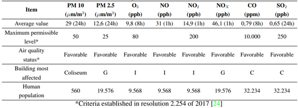
There is a particulate matter concentration of 29 µg/m3 of PM10 in the coliseum and 12,6 µg/m3 of PM2,5 in building G, in addition to 9,8 ppb of O3 in building I, 14,9 ppb of NO2 in that same building, 0,79 ppb of CO in building C, and 0,65 ppb of SO2 also in building C, thus allowing to infer, according to the Bogotá air quality index, a favorable air quality for a population of 2.131 people who visited the campus university during the aforementioned period.
Conclusions:
The correct integration of the data in the web server and their analysis, carried out in the R language, allowed determining the approximate indicators of the polluting factors around Escuela Colombiana de Ingeniería Julio Garavito. Additionally, to determine the affected population, these indicators were correlated with the information on the registered population that entered the campus during the period under study. Based on the results obtained, it was concluded that the air quality on the campus of Escuela Colombiana de Ingeniería Julio Garavito is favorable, and that 2.131 people benefited daily from these conditions.
Keywords:
polluting factors, modeling, Kriging method, air quality, area, population..Resumen
Contexto:
La evaluación de la calidad del aire en Colombia es localizada; no va más allá de determinar si el nivel del gas contaminante en un punto específico de la red de monitoreo ha excedido un umbral, de acuerdo con una norma o estándar, con el fin de generar una alarma. No se compromete con objetivos tan importantes como identificar en tiempo real la dinámica de dispersión de los gases contaminantes en una zona, ni la predicción de la nueva población afectada. Desde esta perspectiva, se evaluó la presencia de los gases contaminantes en el campus universitario de la Escuela Colombiana de Ingeniería Julio Garavito, ubicada al norte de la ciudad de Bogotá, y se estimó la población afectada para el mes de octubre de 2019 utilizando la técnica geoestadística de Kriging.
Método:
Este estudio forma parte del diseño y construcción de una estación móvil auxiliar que monitorea y reporta información complementaria (gases CO y SO2) a la que brinda la estación meteorológica de Guaymaral, ubicada en el norte de Bogotá. Esta información es transmitida a través de una red IoT hacia un servidor, donde se crea una base de datos que almacena la información de los gases contaminantes reportada por las 14 estaciones de la red de monitoreo de calidad del aire de Bogotá, la información enviada por la estación auxiliar y la información estadística de la población presente en el campus universitario. Los datos de los gases contaminantes y la información de la población registrada desde el 1 al 31 de octubre de 2019 son el insumo para el análisis de datos mediante el método de interpolación de Kriging y la predicción de la población afectada en dicho campus.
Resultados:
Se encuentra una concentración de material particulado de 29 µg/m3 de PM10 en el coliseo y 12,6 µg/m3 de PM2,5 en el edificio G. Además de 9,8 ppb de O3 en el edificio I, 14,9 ppb de NO2 en ese mismo edificio, 0,79 ppb de CO en el edificio C y 0,65 ppb de SO2 también en el edificio C, permitiendo inferir, según el índice de calidad del aire de Bogotá, una calidad del aire favorable para una población de 2.131 personas que visitaron el campus universitario durante el período mencionado.
Conclusiones:
La correcta integración de los datos en el servidor web y el análisis de estos, realizado en lenguaje R, permitieron determinar los indicadores aproximados de los factores contaminantes en el área de la Escuela Colombiana de Ingeniería Julio Garavito. Adicionalmente, para determinar la población afectada, estos indicadores se correlacionaron con la información de la población registrada que ingresó al campus durante el periodo de estudio. Con base en los resultados obtenidos, se pudo concluir que la calidad del aire en el campus universitario de la Escuela Colombiana de Ingeniería Julio Garavito es favorable y 2.131 personas se beneficiaron diariamente de estas condiciones.
Palabras clave:
factores contaminantes, modelación, método de Kriging, calidad del aire, área, población..Introduction
In Colombia, the monitoring and control of atmospheric pollution have become increasingly relevant, given that the indicators of atmospheric pollution have peaked in the main cities due to the growth of the industrial sector, the overexploitation of natural resources (coal, wood, etc.), and the increase in the use of vehicles. However, there is still a lack of awareness of this impact, and the necessary administrative instruments and mechanisms for the prevention and control of environmental deterioration factors have not been defined and regulated. Additionally, the evaluation of air quality is motivated by the need to determine whether a norm or standard has been violated, leaving aside another objective, which is to determine the affected population and the risk to human health that may be caused by exposure to pollutants in the atmosphere In this context, the research problem addressed in this paper is the determination of the level of pollution and the affected human population in Escuela Colombiana de Ingeniería Julio Garavito (case study), located in Bogotá, during October 2019. This research was conducted in the campus of the aforementioned educational institution, where the climatological station of Guaymaral operates, which belongs to the Air Quality Monitoring Network of Bogotá (RMCAB). This station detects and reports the values of PM10, PM2,5, O3, NO, NO2, and NOX levels to a centralized database. However, it does not report information on the polluting gases CO and SO2. To determine the level of pollution by recording the eight polluting gases, as well as the affected population in this area, it was necessary to design and build a mobile station that detects CO and SO2 with lowcost sensors, which transmits the information through an Internet of Things (IoT) network with LoRa (Long-Range Protocol) devices and LPWAN (Low-Power WAN) technology to a server. The methodological design for recording (measurements of polluting gases: average values, sampling frequencies, etc.), analysis, and interpretation of the data was based on the guidelines of the protocol for monitoring air quality in Colombia [1]. The contributions of this work are: 1) disclosing pollution levels to a population that works and studies in a specific area in order to take measures to reduce exposure or reassure the academic community, 2) provide new comprehensive technical elements to improve air quality man- agement, and 3) present the results obtained and the methodology followed in this case study to the Colombian Ministry of Environment and Sustainable Development, which seeks to design a national air quality modeling guide.
Theoretical framework
The first works on air quality measurement in Colombia refer to the design of interfaces for the capture of meteorological data and the installation and start-up of this type of station in some cities. At present, the measurements and reporting of the average values of the variables that determine air quality in urban areas, the cut-off points, and the quality index of the network of stations follow the guidelines of the protocol for monitoring air quality [1].
State of the art in the Colombian context
In 2019, the monitoring of atmospheric pollution phenomena in Colombia was carried out with 203 monitoring stations distributed in 83 municipalities and 22 departments. For the case of Bogotá, it was carried out by the District Secretariat of the Environment (SDA) with the RMCAB, which has 14 monitoring stations, out of which 12 are fixed, one is meteorological, and the other one is mobile. This level IV Air Quality Monitoring System (SVCA) is located at strategic sites in the city. The stations have automatic equipment that continuously and permanently monitors concentrations of criteria pollutants, such as particulate matter (PM10, PM2,5) and pollutant gases (O3, CO, NO2, and SO2) and meteorological variables such as precipitation, wind speed and direction, temperature, solar radiation, relative humidity, and barometric pressure.
In the above scenario, Guaymaral is a climatological station of the RMCAB [1] that, according to the National Station Catalog (CNE) of the Institute of Hydrology, Meteorology, and Environmental Studies (IDEAM), is located at 4° 47’ 1,52"north latitude and 74° 2’ 39,06"west longitude, at 2.580 m above sea level in the locality of Suba, northern Bogotá (Fig. 1). This station measures common meteorological variables such as air temperature, precipitation, humidity, wind direction and speed, solar radiation and evaporation, and pollutant gases: PM10, PM2,5, O3, NO, NO2, and NOX. Observations are carried out daily at 7 a.m., 1 p.m., and 7 p.m. Guaymaral does not report any CO or SO2 data.
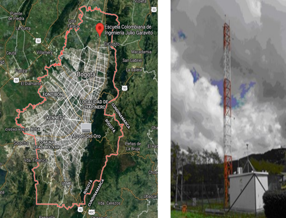
Figure 1: Guaymaral weather station in the locality of Suba, in northern Bogotá, on the campus of the Escuela Colombiana de Ingeniería Julio Garavito
State of the art in the international context
In the international context, the literature on this topic reports information on the most common technologies for wireless sensor interconnection and data transmission from the weather station to the monitoring center. In 2016, [2] proposed a multichannel wireless sensor network with the ZigBee protocol at 2.4 GHz. This study examined the interference between ZigBee and WLAN protocols and sought to improve network performance by increasing the packet delivery rate with the use of time-division multiplexing and cluster tree protocols. [3] developed a monitoring system for a vertical axis wind turbine using ZigBee; monitoring was performed using the LR-WPAN standard, which was compatible with the ZigBee protocol. As for data analysis, data were collected through a layered computing system, which facilitated the integration of sensor information and analysis of the captured data. [4] proposed an environmental gas monitoring system using a sensor array with an SPI output. The research consisted of two parts: a client part and a server part. The latter was written in the C language and had four gas sensors, whereas the client part was programmed as an object in JavaScript, thus facilitating graphical visualization and data analysis. [5] developed a data acquisition system based on the ZigBee and Bluetooth protocols using two Arduino modules: one to read the signals acquired by the sensors and transmit them through the ZigBee module, and the other to retrieve the data. In addition, the Bluetooth module was used to communicate with a smartphone and a computer to visualize the data. [6] designed an automatic irrigation system based on a patented algorithm and powered by solar panels. This system used a duplex wireless network with humidity and temperature sensors located in the soil near the plant roots. As a result of the project, it was possible to reduce water consumption by 90 % over 136 days. [7] developed a wireless data acquisition system based on a PIC16F microcontroller, a RF antenna, rechargeable AA batteries, and photovoltaic panels. The acquired data corresponded to those provided by sensors measuring solar radiation, temperature, relative humidity, pressure, wind speed, and direction. Once the data were acquired, they were modulated and transmitted via RF to a base station, which demodulated the information and sent it through a RS 232 interface to a computer for visualization in LabView. [8] developed a wireless sensor network with Zigbee communication. The interface for data acquisition was built with a microcontroller and an ADC, which communicated with the Zigbee module through a conventional asynchronous serial interface. The data retrieved from the Zigbee receiver were sent to a computer for display on a graphical interface programmed in C#. [9] implemented a monitoring network with LoRa WAN networks to measure PM10 and PM2,5 in the town of Santa Maria Degli Angeli in the municipality of Assis (Italy). For decision making, the multi-criteria AHP technique was used to define the initial positioning of the sensors. As a result, it was found that the largest emitter of pollutants is the industry, followed by urban traffic and domestic heating. [10] used MQ-135 and DHT11 sensors for the detection of CO, CO2, alcohol, air temperature, and humidity, and transmission through an IoT network composed of an Arduino UNO and a Raspberry Pi. As a result, a platform for monitoring and issuing early warnings of the monitored air quality was configured. [11] used the MQ-135 sensor, an Arduino UNO, ESP8266 wifi, and GPS modules to measure and report air quality information via IoT networks to Web GIS clients. The goal of the project was to trigger alarms when the set safety limits were exceeded, and action was taken when the authority failed to minimize pollutant levels after a specified period. [12] detected PM10, PM2,5, temperature, and humidity, and they developed a protocol for the transmission of georeferenced data via a LoRaWAN network. [13] measured CO2 and PM2,5 in the cafeteria kitchen and laboratory room of the Department of Science and Technology of the University of Rwanda. As a result, up to 800 ppm CO2 and 100 ppm PM2,5 were obtained in the kitchen environment, and 500 ppm CO2 and 0 ppm PM2,5 in the laboratory, over an observation time of 11 months.
The above allows inferring that most studies revolve around the design and implementation of sensor networks with technologies such as ZigBee, Wi-Fi, Bluetooth, GPRS, LoRa Wan for environmental monitoring (ESN, Environmental Sensor Networks), and meteorological stations can be located within this category [14]. Although this research designs and builds an auxiliary mobile station (for CO and SO2 detection), and an IoT network composed of nodes (End-Devices), a gateway, a LoRa to IP protocol conversion module (Backhoult), and a database, its interest is focused on data analytics, real-time identification of the dispersion dynamics of pollutant gases, and determining the affected population in a specific area and time (case study).
IoT (The Internet of Things)
IoT is a line-of-sight, low power consumption wide-area protocol network with a coverage of up to 15 km used in various applications in the 2.4 GHz band (unlicensed Industrial, Scientific, and Medical radio bands, ISM) [15]. The LoRa WAN standard protocol has three layers (physical or transmission layer, MAC medium access layer, and application layer) for the transmitting information at a data rate between 0,3 and 50 Kbps [16], [17].
R studio and Kriging interpolation method:
R is a free programming language and a study environment with a statistical approach and graphic features. Kriging is a geostatistical interpolation procedure that includes autocorrelation, i.e., statistical relationships of the data from the measured points. Because of this, not only can it produce an estimated surface from a set of sparse points with z-values, but it also provides some measure of certainty or accuracy. Kriging assumes that the distance or direction between sample points reflects a spatial correlation, which can be used to explain the variation on the surface [18]. This procedure fits a mathematical function to a specific number of points or all points within a specific radius, in order to determine the output value for each location. This is a multi-step process, which includes exploratory statistical analysis of data, variogram modeling, surface creation, and, optionally, the exploration of a variance surface. Kriging is the most appropriate method when a correlated spatial distance or directional bias is known to exist in the data [19]. It is often used in soil science and geology. However, it shows limitations because it does not consider wind direction and speed, terrain topography, and the existence of buildings in the area. For this reason, it is necessary to have many measurement points to correctly estimate the distribution of pollutant gas in the study area.
Materials and methods
The methodological focus is Top-Down, and the approach of this research, according to [20] p. 120, is classified as qualitative, given that “an attempt is made to explain and predict the phenomena investigated, looking for regularities and causal relationships between elements". Besides, according to the same source, a subcategory of this research can be established as quantitative correlational, since the purpose is "to know the relationship or degree of association that exists between two or more concepts, categories, or variables in a particular context", in the case of this research, the real-time monitoring and evaluation of air quality in an area of Bogotá.
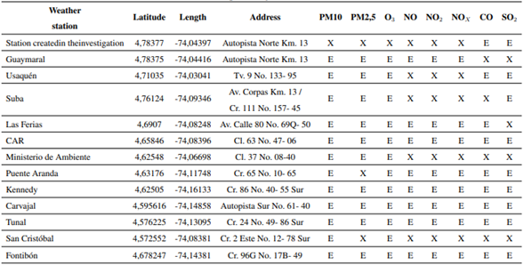
In this context, not all RMCAB weather stations report all the polluting factors (particulate matter, gases, and meteorological variables that are necessary to assess the pollutant dispersion dynamics, and thus determine the affected areas and population (Table I).
Table I: Measurement of polluting factors in the weather stations
One of the exposed cases is the Guaymaral meteorological station, which lacks the sensors to monitor carbon monoxide (CO) and sulfur dioxide (SO2). For this reason, an auxiliary station was designed and built for said station, which was installed between September 29th and November 1st , 2019. It was placed 5 m north of it, and it was interconnected to a server for data transmission over an IoT network. This network was designed and built with a PIC family microchip, as shown in Fig. 2.

Figure 2: Auxiliary station connected to the server through the IoT network
The MQ-136 and MQ-7 sensors were chosen to measure the SO2 and CO concentration levels. The first of these works with 5 V and has a high SO2 detection sensitivity (Fig. 3, blue line), between 1 and 100 ppm, with an accuracy of 0,65 % at a temperature of 20 ± 2 °C and relative humidity of 65 ± 5 %. The calibration of this sensor was carried out with calibration gases with a concentration of 10 ppm. Later, these values were compared with those of the RMCAB weather station, where an error of 8,7 % was found. Fig. 3 shows the response curve of the MQ-136 sensor against different gases, where cross-sensitivities to various gases are evident.
![Typical sensitivity characteristics of the MQ-136 sensor for various gases at a temperature of 20 °C, relative humidity of 65 %, O2 concentration of 21 %, RL = 20 kΩ. R0: resistance of the sensor to 10 ppm of SO2 in clean air; Rs: resistance of the sensor to various concentrations of gases [21]](https://revistas.udistrital.edu.co/index.php/reving/article/download/17589/version/13253/17938/112355/0121-750X-inge-26-03-401-gf3.png)
Figure 3: Typical sensitivity characteristics of the MQ-136 sensor for various gases at a temperature of 20 °C, relative humidity of 65 %, O2 concentration of 21 %, RL = 20 kΩ. R0: resistance of the sensor to 10 ppm of SO2 in clean air; Rs: resistance of the sensor to various concentrations of gases [21]
On the other hand, the second sensor also works with 5 V and has a detection sensitivity between 20 and 2.000 ppm of CO, with an accuracy of 0,5 % (Fig. 4, violet line). This, at the same temperature of 20 ± 2 °C and relative humidity of 65 ± 5 %. The calibration of these sensors was carried out as follows: the information provided by the station created in this investigation was compared with that reported by one of the RMCAB meteorological stations (standard sensor). For this, the station created was placed at 3 m from the RMCAB station, and 3 m from the ground for a period of 8 hours. The values obtained were compared with each other: an error of 8,7 % for SO2 and an error of 3,4 % for CO. These values were used to adjust the test sensor with the value reported by the standard one. Fig. 4 shows the response curve of the MQ-7 sensor against different gases that have a lower Rs/Ro ratio, high sensitivity to CO, and a medium sensitivity to H2. The MQ-7 allows us to accurately measure CO.
![Typical sensitivity characteristics of the MQ-7 sensor for various gases at a temperature of 20 °C, relative humidity of 65 %, and O2 concentration of 21 %, RL = 10 kω. R0: resistance of the sensor to 100 ppm of SO2 in clean air; Rs: resistance of the sensor to various concentrations of gases [22]](https://revistas.udistrital.edu.co/index.php/reving/article/download/17589/version/13253/17938/112356/0121-750X-inge-26-03-401-gf4.png)
Figure 4: Typical sensitivity characteristics of the MQ-7 sensor for various gases at a temperature of 20 °C, relative humidity of 65 %, and O2 concentration of 21 %, RL = 10 kω. R0: resistance of the sensor to 100 ppm of SO2 in clean air; Rs: resistance of the sensor to various concentrations of gases [22]
The information acquired by the sensors was sent to the IoT node. This node communicated with the gateway, which was implemented in a Raspberry Pi and programmed in Python to convert the LoRa protocol frames to IP. From the gateway, the information was transmitted to a server through the cloud, which was geographically located within the same city but at another university. The CO and SO2 data measured by the SDA of the Guaymaral station, as well as that sent by the auxiliary station, were stored in this equipment and visualized through a graphical interface called "Grafana"(Fig. 2).
The transmission of the information was carried out through bidirectional time slots from the application layer, obeying the following steps: the node requests a login (entry) to the network with the configuration data and opens a reception window (listening mode). The gateway receives the request and sends it to the server, which verifies that the node is registered and the encryption key is correct. If the data are correct, it allocates a temporary session and sends it through the Gateway to the node. If they are wrong, it rejects the combination. The node receives the temporary session and can send data to the network according to a defined schedule.
For data analytics, a database was generated on a server for geo-referencing of the Guaymaral station’s monitoring point (Geographic Information Systems, GIS, were used). This database stored the information (in HTML format) of the polluting factors that were reported by the Guaymaral climatological station in the period from October 1st to 31st. Subsequently, the data from the Guaymaral station were compiled and later converted into a tabular format [23]. This information, along with the data received from the auxiliary station, was organized by averaging the data from each sensor in the recorded period, leaving a single geo-referenced value for each gas in each meteorological station, and it was finalized as the input of the data analytics.
The analysis includes data represented in tables and graphs with a comparison of daily hourly averages (every 1,8 and 24 hours, as well as mobile 8-hour averages, as appropriate) and an evaluation with the maximum permissible levels according to the exposure times established in national regulations (Resolution 2.254 of 2017 of the Ministry of Environment and Sustainable Development, MADS). The calculation of each average considers a temporal coverage of at least 75 % of the data.
The spatial distribution of the pollutant concentration measurements is represented by spatial interpolation maps resulting from the implementation of the Kriging geostatistical method, which uses the R Studio software. Therefore, it should be noted that these representations are subject to the presence of uncertainties, which are typical of a procedure that seeks to obtain secondary information based on the measurements of the mobile auxiliary station and each RMCAB station.
The procedure is shown in the flow diagram of Figure 5, which consists of selecting the polluting factor, along with its corresponding average value, that is geographically reported by each weather station in the city of Bogotá. These data and the points of the geographical location of the stations are used to construct a frequency histogram, evaluate their normality, and calculate the semi-variance in order to determine the most appropriate statistical model to predict the polluting factor. Finally, the Kriging interpolation is performed, the dispersion dynamics of the pollutant factor in the area is graphically obtained, and the local monitoring area is zoomed (Escuela Colombiana de Ingeniería Julio Garavito, ECIJG) with a spatial resolution of 10 m. With the above, the indicators of the polluting factors are obtained at a local level.

Figure 5: Procedure to obtain the statistical prediction model
Fig. 6 shows an example of the steps followed to determine the dispersion of PM10 particulate material and the results obtained. The frequency histogram for PM10 is constructed with the average data that were recorded and reported every 24 hours by the weather stations of Bogotá. The semi-variance graph approximates a statistical model according to the distribution of the data, which represent groups of distances existing between the location points of the Bogotá weather stations (discarding extreme distances greater than 30 km and close to 0 m or null distance, in which the particulate material does not show any changes).
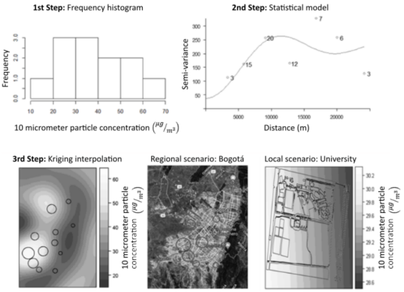
Figure 6: Steps followed to determine the presence of PM10 particulate matter in the university
Then, the prediction model is adjusted, and the Kriging interpolation is performed, which gives a graph in contour lines of the concentration of PM10 in a domain mesh of the regional model. The concentration isopleths of this particulate material are obtained locally, and the domain mesh is limited with a resolution of 10 m to achieve a spatial zoom.
The procedure was the same for the rest of the polluting factors, namely the concentration of PM2,5 particulate matter and polluting gases SO2, NO2, CO, and O3. The parameterization of the academic and administrative community of ECIJG, which was present in each of the university buildings, was carried out in time slots (according to class changes), for a normal daytime schedule from 7:00 a.m to 7:00 p.m, and for the period from October 1st to 31st, 2019. The sources of information were the registration and human resources offices of the same university. Fig. 7 shows a sample of the presence of the university population in one of the campus buildings, specifically building D.

Figure 7: Average number of people present from October 1st to 6th, 2019 at the facilities of building D of ECIJG
Results
Fig. 8 shows the results of the demographic study of the number of people per week and per building on the university campus of ECIJG for the period under study. The average number of people per day staying overnight at the university campus was 2.131 for the same period.

Figure 8: Distribution of the average human population on the university campus
Fig. 9 shows the concentration of particulate matter PM10, PM2,5, and pollutant gases SO2, NO2, CO, and O3 found on the university campus during an average day within the period indicated above.

Figure 9: Distribution of a) PM10 (µg /m3), b) PM2,5 (µg /m3), c) CO (ppm), d) O3 (ppb), e) NO (ppb), f) NO2 (ppb), g) NOX (ppb), and h) SO2 (ppb), in ECIJG
Table II shows the average level of each pollutant factor, the maximum permissible levels, the state of air quality by building, and the population.
Table II: Indicators of contaminating factors at ECIJG from October 1st to 31st, 2019
The monthly average concentrations of PM10 and PM2,5 during October 2019 showed a similar behavior to the annual report by the environmental control directorate of the district environmental secretariat concerning spatial distribution [1]. The highest concentrations were maintained in the southwest (colosseum) and northeast (building G) of the campus and the lowest in the northeast and southwest areas, respectively. In comparison with the concentrations of previous years of the same report [1], for PM10, there is a tendency for concentrations to decrease over time, but PM2,5 concentrations tend to increase.
Monthly concentrations of PM2,5 and PM10 are influenced by variations in the meteorology of each month of the year. The first quarter is characterized by being a dry period, so there is a re duction in wind speed and a greater frequency of thermal inversions. In the second quarter, the rainy season begins, which favors the decrease in concentrations to some extent. The second dry season coincides with September and October, in which concentrations increase again to decrease in December due to the reduction in the activity of several emission sources.
During a typical day, concentrations are low in the early morning, and they increase rapidly until reaching a peak between 7 and 8 a.m. due to the beginning of activity at the emission source, mainly associated with vehicle traffic on the city’s northern highway. Because the temperature difference between day and night at the surface is greater in the morning hours, the dispersion of pollutants is low. However, as the day progresses, the surface temperature increases, which favors wind speed and the dispersion of pollutants during the rest of the day. In the afternoon, a slight increase in concentrations is observed, which is associated with vehicle activity at the end of the workday.
The mobile station built during this project monitored CO during October 2019. It recorded valid data in a percentage higher than 65 %. Building C showed the highest average, with 0,79 ppb, and building F recorded the lowest monthly concentration. On an average day, CO concentrations are highest in the morning between 6 and 8 a.m. as well as during the late afternoon and evening, between 5 and 10 p.m. The lowest concentrations are recorded around noon. CO concentrations in 2019 increased at some RMCAB stations relative to previous years, although there was a slight decrease for that year at stations in the southwest. It was observed that the buildings on the university campus - located near the northern highway - are the ones with the highest CO levels, especially due to the influence of the older vehicle fleet. Concerning the maximum permissible levels established by the standard, no exceedances of the hourly and 8-hour moving average data were recorded during 2019.
Building I, located in the southwestern sector of the university campus, recorded the highest monthly average of O3, with 9,8 ppb, whereas building G recorded the lowest levels. The behavior of this pollutant has varied over the years, although, historically, the north of the city (the area where ECIJG is located) has recorded the highest concentrations [1]. The harmful tropospheric ozone (O3) that exists in the lower layers is not emitted directly into the atmosphere but is produced by the chemical reaction between natural oxygen in the air and nitrogen oxides and hydrocarbons, which act as precursors or facilitators of the chemical reaction in the presence of sunlight. These precursors are emitted directly into the atmosphere; the higher the concentration of these precursors, the higher the ozone production, provided that solar radiation is present. Concentration levels are influenced by the variation of solar radiation during the day, with the highest peaks occurring around 1 p.m. In the morning, concentrations are low, decreasing around 6 a.m., influenced by the increase in NO2 concentrations, increasing until they peak in the afternoon, and decreasing again after the reduction of solar radiation.
The average week’s ozone behavior starts with high concentrations on Monday and decreases until Wednesday. There is a slight increase on Thursday, and a decrease towards Saturday, with a sharp increase on Sunday. Because O3 is a secondary pollutant, variations in concentration are determined by the concentrations and magnitude of O3 precursor factors, such as the variation in solar radiation during the year, which predominates in dry seasons, or changes in NO2 and VOC concentrations.
The highest NO2 concentrations were recorded in the southwest of the university campus, in building I, with 14,9 ppb, and the lowest concentrations were obtained in buildings F and G. No exceedances of the maximum limits were recorded at both annual and hourly resolutions. Concerning previous years, concentrations have remained similar in most stations since 2015 [15]. The highest concentrations predominate in March and April, decrease in the middle of the year, and increase again between September and October. The variation in NO2 concentrations coincides with periods of high concentration of particulate matter, since the impact of emissions from combustion processes is more noticeable in the dry season, given that the dispersion capacity of the concentrations is reduced. Concentrations are lowest on Monday, and they gradually increase on Wednesday and then decrease in the following days until Saturday, when the highest concentrations of the week occur. The increase in concentration on weekdays may be influenced by the accumulation of pollution during the week, in addition to chemical reactions occurring in the atmosphere. On Saturdays, there are no mobility restrictions for vehicles, so there may be increases in concentrations due to emissions associated with mobile sources.
In 2019, the highest annual average of SO2 was recorded in building C with a value of 0,65 ppb. This behavior is influenced by the activity of emission sources during the week (a vehicle fleet with greater use of diesel circulates along the northern highway, both with freight and public transport), as well as on weekends, since there is increased traffic due to the departure of vehicles from the city. No exceedances of the daily limit were recorded. In general, since 2015, there have been slight reductions in concentrations over the years in most of the RMCAB stations [1].
However, the concentration levels of particulate matter and pollutant gases, which were specified in Table II and affect a floating population per building on the campus of ECIJG, allow classifying the average air quality as favorable according to IBOCA, as well as stating that it meets the environmental criteria [25].
Discussion
The results presented in the previous section allow inferring that 2.131 people benefit daily from the favorable state of air quality in the facilities of ECIJG. Similarly, it is concluded that the pollutant with the greatest potential for affecting the university campus is particulate matter of less than 2,5 microns (PM2,5), a result that coincides with that reported by the SDA [26] for Bogotá. It is recommended that members of the academic community, among other measures, use public transportation or opt for bicycles for commuting from their homes to the institution and vice-versa. Wet sweeping (general services) is also recommended, and vehicle users should avoid filling the gas tank of the car to the maximum to contribute to maintaining or improving air quality on campus.
Additionally, it is necessary for Colombia to evaluate the coverage of its weather stations to know if their number and distribution throughout the territory are sufficient and adequate to monitor the quality of the air that its citizens breathe. In the specific case of the RMCAB, it is recommended that the number be increased to cover the entire urban area, and that some of the existing stations be equipped with the necessary equipment to measure all pollutant factors. Similarly, a reevaluation the limits established by the Colombian standard for determining air quality should be carried out because it is laxer than the one suggested by the World Health Organization (WHO). For example, while the Colombian limit for PM10 is 50 µg/m3, the WHO recommendation is 20 µg/m3.
With the increase in the number of measurement points in a reduced area, future work could focus on determining specific places that are not complying with health regulations and send a timely warning to the population, analyzing the data with unsupervised learning in real time.
Considering the relationship of more variables in the dispersion of the gases, it is also possible to look for an interpolation model in which parameters such as prevailing winds (and their intensities), orography, and buildings are considered to find better gas distribution approximations.
Conclusions
The air pollutant emission inventory for the university campus of ECIJG during October 2019 allowed quantifying the emissions of a specific area (which is ideal to have a general overview of the state of emissions at the city level) generated by different pollutant sources. It provided technical information that serves the environmental authority for the following purposes: a diagnostic tool to manage the air quality of a part of the Suba locality, technical support for the formulation of policies and strategies to mitigate pollution, input information to evaluate the effectiveness of actions through air quality modeling, and the periodic generation of air quality forecasts, among other purposes.
In this type of studies, it is important that the measurement of the values of air pollution factors, in the case of this research, CO and SO2, be carried out with the same criteria established by the Ministry of Environment and the regional governments in order to avoid different reports that confuse citizens. This type of exercise provides baseline data for air preservation policies.
From the study, it can be concluded that the air quality in ECIJG is favorable and that 2.131 people benefit daily from these conditions. On the other hand, the implemented IoT network complies with the conditions of correct transmission and real-time information retrieval. This was validated in the server with the measured values of carbon monoxide and sulfur dioxide, which were previously measured and sent from the monitoring point.
The correct integration of the data in the web server, as well as their analysis performed in the R language, allowed determining the approximate indicators of the polluting factors in the reference area of the university campus of ECIJG, which was correlated with the population occupying its facilities from October 1st to 31st, 2019, in order to determine the affected population.
Acknowledgements
Acknowledgment
This work has been supported by Escuela Colombiana de Ingeniería Julio Garavito and Universidad Distrital Francisco José de Caldas, both located in Bogotá D.C., Colombia, which funded the project with code PRY19.
References
Licencia
Derechos de autor 2022 Hernán Paz Penagos, Andrés Alejandro Moreno Sánchez, José Noé Poveda Zafra

Esta obra está bajo una licencia internacional Creative Commons Atribución-NoComercial-CompartirIgual 4.0.
![]()
A partir de la edición del V23N3 del año 2018 hacia adelante, se cambia la Licencia Creative Commons “Atribución—No Comercial – Sin Obra Derivada” a la siguiente:
Atribución - No Comercial – Compartir igual: esta licencia permite a otros distribuir, remezclar, retocar, y crear a partir de tu obra de modo no comercial, siempre y cuando te den crédito y licencien sus nuevas creaciones bajo las mismas condiciones.

2.jpg)