DOI:
https://doi.org/10.14483/23448393.17973Publicado:
2022-01-04Número:
Vol. 27 Núm. 1 (2022): Enero-AbrilSección:
Ingeniería MecánicaCharacterization, Design Testing and Numerical Modeling of a Subsonic-Low Speed Wind Tunnel
Caracterización, pruebas de diseño y modelado numérico de un túnel de viento subsónico de baja velocidad
Palabras clave:
túneles de viento, Método de Elementos Finitos, flujo irrotacional (es).Palabras clave:
wind tunnels, Finite Element Method, irrotational flow (en).Descargas
Referencias
M. Freydin, E. H. Dowell, S. M. Spottswood, and R. A. Perez, “Nonlinear dynamics and flutter of plate and cavity in response to supersonic wind tunnel start,” Nonlinear Dynamics, vol. 103, no. 4, pp. 3019–3036, 2021. DOI: https://doi.org/10.1007/s11071-020-05817-x
N. Tabatabaei, R. Örlü, R. Vinuesa, and P. Schlatter, “Aerodynamic free-flight conditions in wind tunnel mod- ¨ elling through reduced-order wall inserts,” Fluids, vol. 6, no. 8, p. 265, 2021. https://doi.org/10. 3390/fluids6080265 DOI: https://doi.org/10.3390/fluids6080265
D. Khan, J. H. Bjernemose, I. Lund, and J. E. Bebe, “Design and construction of an open loop subsonic high temperature wind tunnel for investigation of scr dosing systems,” International Journal of Thermofluids, vol. 11, p. 100106, 2021. https://doi.org/doi.org/10.1016/j.ijft.2021.100106 DOI: https://doi.org/10.1016/j.ijft.2021.100106
M. Hand, D. Simms, L. Fingersh, D. Jager, J. Cotrell, S. Schreck, and S. Larwood, “Unsteady aerodynamics experiment phase vi: wind tunnel test configurations and available data campaigns,” tech. rep., National Renewable Energy Lab., Golden, CO.(US), 2001. DOI: https://doi.org/10.2172/15000240
U. Saha, S. Thotla, and D. Maity, “Optimum design configuration of savonius rotor through wind tunnel experiments,” Journal of Wind Engineering and Industrial Aerodynamics, vol. 96, no. 8-9, pp. 1359–1375, 2008. DOI: https://doi.org/10.1016/j.jweia.2008.03.005
B. M. Simmons and P. C. Murphy, “Wind tunnel-based aerodynamic model identification for a tilt-wing, distributed electric propulsion aircraft,” in AIAA SciTech 2021 Forum, p. 1298, 2021. https://doi.org/10. 2514/6.2021-1298 DOI: https://doi.org/10.2514/6.2021-1298
R. C. Busan, P. C. Murphy, D. B. Hatke, and B. M. Simmons, “Wind tunnel testing techniques for a tandem tilt-wing, distributed electric propulsion vtol aircraft,” in AIAA SciTech 2021 Forum, p. 1189, 2021. https://doi.org/10.2514/6.2021-1189 DOI: https://doi.org/10.2514/6.2021-1189
Y.-D. Huang, N. Xu, S.-Q. Ren, L.-B. Qian, and P.-Y. Cui, “Numerical investigation of the thermal effect on flow and dispersion of rooftop stack emissions with wind tunnel experimental validations,” Environmental Science and Pollution Research, vol. 28, no. 9, pp. 11618–11636, 2021. https://doi.org/10.1007/s11356-020-11304-y DOI: https://doi.org/10.1007/s11356-020-11304-y
C. A. Banach, A. M. Bradley, R. G. Tonkyn, O. N. Williams, J. Chong, D. R. Weise, T. L. Myers, and T. J. Johnson, “Dynamic infrared gas analysis from longleaf pine fuel beds burned in a wind tunnel: observation of phenol in pyrolysis and combustion phases,” Atmospheric Measurement Techniques, vol. 14, no. 3, pp. 2359– 2376, 2021. https://doi.org/10.5194/amt-14-2359-2021 DOI: https://doi.org/10.5194/amt-14-2359-2021
C. Ocker, E. Blumendeller, P. Berlinger, W. Pannert, and A. Clifton, “Localization of wind turbine noise using a microphone array in wind tunnel measurements,” Wind Energy, 2021. https://doi.org/10.1002/we.2665 DOI: https://doi.org/10.1002/we.2665
E. Gnapowski, J. Pytka, J. Józwik, J. Laskowski, and J. Michałowska, “Wind tunnel testing of plasma actuator with two mesh electrodes to boundary layer control at high angle of attack,” Sensors, vol. 21, no. 2, p. 363, 2021. https://doi.org/10.3390/s21020363 DOI: https://doi.org/10.3390/s21020363
Š. Nosek, Z. Jaňour, D. Janke, Q. Yi, A. Aarnink, S. Calvet, M. Hassouna, M. Jakubcová, P. Demeyer, and G. Zhang, “Review of wind tunnel modelling of flow and pollutant dispersion within and from naturally ventilated livestock buildings,” Applied Sciences, vol. 11, no. 9, p. 3783, 2021. https://doi.org/10.3390/act10060107 DOI: https://doi.org/10.3390/app11093783
M. J. E. Yazdi and A. B. Khoshnevis, “Experimental study of the flow across an elliptic cylinder at subcritical reynolds number,” The European Physical Journal Plus, vol. 133, no. 12, p. 533, 2018. https://doi.org/10.1140/epjp/i2018-12342-1 DOI: https://doi.org/10.1140/epjp/i2018-12342-1
S. Bryson and C. Levit, “The virtual wind tunnel,” IEEE Computer graphics and Applications, no. 4, pp. 25–34, 1992. DOI: https://doi.org/10.1109/38.144824
S. K. Reinhardt, M. D. Hill, J. R. Larus, A. R. Lebeck, J. C. Lewis, and D. A. Wood, “The wisconsin wind tunnel: virtual prototyping of parallel computers,” in Proceedings of the 1993 ACM SIGMETRICS conference on Measurement and modeling of computer systems, pp. 48–60, 1993. DOI: https://doi.org/10.1145/166962.166979
J. Counihan, “An improved method of simulating an atmospheric boundary layer in a wind tunnel,” Atmospheric Environment (1967), vol. 3, no. 2, pp. 197–214, 1969. DOI: https://doi.org/10.1016/0004-6981(69)90008-0
M. Tang, M. Böswald, Y. Govers, and M. Pusch, “Identification and assessment of a nonlinear dynamic actuator ¨ model for gust load alleviation in a wind tunnel experiment,” CEAS Aeronautical Journal, 2021. https://doi.org/10.1007/s13272-021-00504-y DOI: https://doi.org/10.1007/s13272-021-00504-y
B. H. Goethert, “Transonic wind tunnel testing,” tech. rep., ADVISORY GROUP FOR AERONAUTICAL RESEARCH AND DEVELOPMENT PARIS (FRANCE), 1961.
J. Kendall, “Wind tunnel experiments relating to supersonic and hypersonic boundary-layer transition,” Aiaa Journal, vol. 13, no. 3, pp. 290–299, 1975. DOI: https://doi.org/10.2514/3.49694
M. Costantini, T. Lee, T. Nonomura, K. Asai, and C. Klein, “Feasibility of skin-friction field measurements in a transonic wind tunnel using a global luminescent oil film,” Experiments in Fluids, vol. 62, no. 1, pp. 1–34, 2021. https://doi.org/10.1007/s00348-020-03109-z DOI: https://doi.org/10.1007/s00348-020-03109-z
D. T. Reese, R. J. Thompson, R. A. Burns, and P. M. Danehy, “Application of femtosecond-laser tagging for unseeded velocimetry in a large-scale transonic cryogenic wind tunnel,” Experiments in Fluids, vol. 62, no. 5, pp. 1–19, 2021. https://doi.org/10.1007/s00348-021-03191-x DOI: https://doi.org/10.1007/s00348-021-03191-x
L. P. Chamorro and F. Porté-Agel, “A wind-tunnel investigation of wind-turbine wakes: boundary-layer turbulence effects,” Boundary-layer meteorology, vol. 132, no. 1, pp. 129–149, 2009. DOI: https://doi.org/10.1007/s10546-009-9380-8
L. Mydlarski and Z. Warhaft, “On the onset of high-reynolds-number grid-generated wind tunnel turbulence,” Journal of Fluid Mechanics, vol. 320, pp. 331–368, 1996. DOI: https://doi.org/10.1017/S0022112096007562
K. Inokuma, T. Watanabe, K. Nagata, and Y. Sakai, “Statistical properties of spherical shock waves propagating through grid turbulence, turbulent cylinder wake, and laminar flow,” Physica Scripta, vol. 94, no. 4, p. 044004, 2019. https://doi.org/10.1088/1402-4896/aafde2 DOI: https://doi.org/10.1088/1402-4896/aafde2
A. Alexander and B. Holownia, “Wind tunnel tests on a savonius rotor,” Journal of Wind Engineering and Industrial Aerodynamics, vol. 3, no. 4, pp. 343–351, 1978 DOI: https://doi.org/10.1016/0167-6105(78)90037-5
T. Chen and L. Liou, “Blockage corrections in wind tunnel tests of small horizontal-axis wind turbines,” Experimental Thermal and Fluid Science, vol. 35, no. 3, pp. 565–569, 2011 DOI: https://doi.org/10.1016/j.expthermflusci.2010.12.005
M. S. Selig and B. D. McGranahan, “Wind tunnel aerodynamic tests of six airfoils for use on small wind turbines,” J. Sol. Energy Eng., vol. 126, no. 4, pp. 986–1001, 2004. DOI: https://doi.org/10.1115/1.1793208
H.-J. Rothe, W. Biesel, and W. Nachtigall, “Pigeon flight in a wind tunnel,” Journal of comparative Physiology B, vol. 157, no. 1, pp. 99–109, 1987. https://doi.org/10.1007/BF00702736 DOI: https://doi.org/10.1007/BF00702734
J. Liu, R. Kimura, M. Miyawaki, and T. Kinugasa, “Effects of plants with different shapes and coverage on the blown-sand flux and roughness length examined by wind tunnel experiments,” Catena, vol. 197, p. 104976, 2021. https://doi.org/10.1016/j.catena.2020.104976 DOI: https://doi.org/10.1016/j.catena.2020.104976
A. Lago, D. Trabucco, and A. Wood, “Chapter-7 testing, inspection, and maintenance,” in Damping Technologies for Tall Buildings, pp. 465–531, Butterworth-Heinemann, 2019. https://doi.org/10.1016/B978-0-12-815963-7.00007-5 DOI: https://doi.org/10.1016/B978-0-12-815963-7.00007-5
E. Maskell, “A theory of the blockage effects on bluff bodies and stalled wings in a closed wind tunnel,” tech. rep., Aeronautical Research Council London (United Kingdom), 1963.
L. Cattafesta, C. Bahr, and J. Mathew, “Fundamentals of wind-tunnel design,” Encyclopedia of Aerospace Engineering, pp. 1–10, 2010. https://doi.org/10.1002/9780470686652.eae532 DOI: https://doi.org/10.1002/9780470686652.eae532
M. A. G. Hernández, A. I. M. López, A. A. Jarzabek, J. M. P. Perales, Y. Wu, and S. Xiaoxiao, “Design methodology for a quick and low-cost wind tunnel,” in Wind tunnel designs and their diverse engineering applications, IntechOpen, 2013. https://doi.org/10.5772/54169 DOI: https://doi.org/10.5772/54169
J. B. Barlow, W. H. Rae, and A. Pope, “Low-speed wind tunnel testing,” 1999.
N. Nordin, A. Karim, Z. Ambri, S. Othman, and V. R. Raghavan, “Design and development of low subsonic wind tunnel for turning diffuser application,” in Advanced Materials Research, vol. 614, pp. 586–591, Trans Tech Publ, 2013. https://doi.org/10.4028/www.scientific.net/AMR.614-615.586. DOI: https://doi.org/10.4028/www.scientific.net/AMR.614-615.586
M. Patel and M. Patel, “Design approach to mach number 0.5 low speed subsonic wind tunnel,” Available at SSRN 2015561, 2012. https://doi.org/10.2139/ssrn.2015561 DOI: https://doi.org/10.2139/ssrn.2015561
M. Arifuzzaman and M. Mohammad, “Design construction and performance test of a low cost subsonic wind tunnel,” IOSR Journal of Engineering, vol. 10, pp. 83–92, 2012. https://doi.org/10.9790/3021-021058392 DOI: https://doi.org/10.9790/3021-021058392
F. Acevedo Vélez et al., “Diseño de un túnel de viento para prueba de ventiladores y perfiles aerodinámicos,” B.S. thesis, Universidad EAFIT, 2006.
F. E. C. Molina, “Diseño y construcción de un túnel de viento,” bachelor’s thesis, Universidad Centroamericana José Simeón Cañas, 2012.
P. Fadilah and D. Erawan, “Effect of applying screen and honeycomb to the flow characteristic in wind tunnel based on cfd simulation,” in Journal of Physics: Conference Series, vol. 1130, p. 012008, IOP Publishing, 2018. https://doi.org/10.1088/1742-6596/1130/1/012008 DOI: https://doi.org/10.1088/1742-6596/1130/1/012008
E.-S. Zanoun, “Flow characteristics in low-speed wind tunnel contractions: Simulation and testing,” Alexandria engineering journal, 2017. https://doi.org/10.1016/j.aej.2017.08.024 DOI: https://doi.org/10.1016/j.aej.2017.08.024
V. Vishwanathan, M. Szoke, J. E. Duetsch-Patel, A. Gargiulo, D. J. Fritsch, A. Borgoltz, C. J. Roy, K. T. Lowe, and W. J. Devenport, “Aerodynamic design and validation of a contraction profile for flow field improvement and uncertainty quantification in a subsonic wind tunnel,” in AIAA SciTech 2020 Forum, p. 2211, 2020. https://doi.org/10.2514/6.2020-2211 DOI: https://doi.org/10.2514/6.2020-2211
J. John, E. A. Pane, B. M. Suyitno, G. H. Rahayu, D. Rhakasywi, A. Suwandi, et al., “Computational fluid dynamics simulation of the turbulence models in the tested section on wind tunnel,” A in Shams Engineering Journal, vol. 11, no. 4, pp. 1201–1209, 2020. https://doi.org/10.1016/j.asej.2020.02.012 DOI: https://doi.org/10.1016/j.asej.2020.02.012
C. J. Doolan, “Numerical evaluation of contemporary low-speed wind tunnel contraction designs,” J. Fluids Eng., vol. 129, no. 9, pp. 1241–1244, 2007. https://doi.org/10.1115/1.2771578. DOI: https://doi.org/10.1115/1.2771578
P. Kundu and L. Cohen, “Fluid mechanics, 638 pp,” Academic, Calif, 1990.
J. A. S. Del Rio, J. G. A. Marin, S. V. Garcia, D. M. Londoño, and D. A. H. Zuluaga, “Simulation analysis of a coanda-effect ejector using cfd,” Tecciencia, vol. 12, no. 22, p. 3, 2017. https://doi.org/10.18180/tecciencia.2017.22.3
J. G. Ardila Marín, D. A. Hincapié Zuluaga, and J. A. Casas Monroy, “Comparison and validation of turbulence models in the numerical study of heat exchangers,” Tecciencia, vol. 10, no. 19, pp. 49–60, 2015. http://dx.doi.org/10.18180/tecciencia.2015.19.8 DOI: https://doi.org/10.18180/tecciencia.2015.19.8
J. D. Betancur Gomez, F. Hoyos Gómez, D. Osorio Patiño, J. G. Marín, and J. A. Sierra del Rio, “Comparison of stress concentration curves for different geometries of machine elements obtained via simulation and experimentation,” Tecciencia, vol. 12, no. 23, pp. 93–101, 2017. https://doi.org/10.18180/tecciencia. 2017.23.11 DOI: https://doi.org/10.18180/tecciencia.2017.23.11
C. A. Sanchez-Ríos, J. Graciano-Uribe, S. Velez García, and D. A. Hincapié-Zuluaga, “Comparative analysis between a discrete spiral chamber and a continuous spiral chamber via ansys,” Tecciencia, vol. 12, no. 23, pp. 25–32, 2017. https://doi.org/10.18180/tecciencia.2017.23.4 DOI: https://doi.org/10.18180/tecciencia.2017.23.4
L. F. Villamarín Guerrero, M. A. Mayorga Betancourt, M. C. Amaris Mendoza, M. Herrera Martínez, and D. R. Sánchez Tachack, “Evaluation of the microlocal wind power potential for the operation of a university wind turbine,” Tecciencia, vol. 12, no. 23, pp. 1–8, 2017. https://doi.org/10.18180/tecciencia.2017.23.1 DOI: https://doi.org/10.18180/tecciencia.2017.23.1
C. Bayona-Roa, R. Codina, and J. Baiges, “Variational multiscale error estimators for the adaptive mesh refinement of compressible flow simulations,” Computer Methods in Applied Mechanics and Engineering, vol. 337, pp. 501–526, 2018. https://doi.org/10.1016/j.cma.2018.03.010 DOI: https://doi.org/10.1016/j.cma.2018.03.010
R. P. Salazar, G. Téllez, D. F. Jaramillo, and D. L. González, “Caos en el billar de forma de diamante y corona redondeada,” Revista de la Academia Colombiana de Ciencias Exactas, Físicas y Naturales, vol. 39, pp. 152– 170, jun. 2015. https://doi.org/10.18257/raccefyn.99 DOI: https://doi.org/10.18257/raccefyn.99
C. Bayona, J. Baiges, and R. Codina, “Variational multiscale approximation of the one-dimensional forced burgers equation: The role of orthogonal subgrid scales in turbulence modeling,” International Journal for Numerical Methods in Fluids, vol. 86, no. 5, pp. 313–328, 2018. https://doi.org/10.1002/fld. 4420 DOI: https://doi.org/10.1002/fld.4420
R. Salazar, C. Bayona-Roa, and J. Solís-Chaves, “Electrostatic field of angular-dependent surface electrodes,” The European Physical Journal Plus, vol. 135, no. 1, p. 93, 2020. https://doi.org/10.1140/epjp/s13360-019-00090-3 DOI: https://doi.org/10.1140/epjp/s13360-019-00090-3
J. A. S. Del Rio, J. G. A. Marin, S. V. Garcia, D. M. Londoño, and D. A. H. Zuluaga, “Simulation analysis of a coanda-effect ejector using cfd,” Tecciencia, vol. 12, no. 22, p. 3, 2017. https://doi.org/10.18180/tecciencia.2017.22.3 DOI: https://doi.org/10.18180/tecciencia.2017.22.3
J. Parra and R. Ríos Linares, “Estudio del comportamiento bajo carga de un chasis para transporte de pasajeros por medio de la tecnología de elementos finitos en la empresa equitel cumandes sa,” AVANCES Investigación en Ingeniería, no. 6, pp. 103–109, 2006
J. A. Guerrero, D. C. Martínez, and L. M. Méndez, “Análisis biomecánico comparativo entre coronas individuales y restauraciones ferulizadas implanto soportadas mediante el uso del método de los elementos finitos,” AVANCES: Investigación en Ingeniería, vol. 8, no. 2, pp. 7–17, 2011.
J. M. P. Ballesteros, O. A. G. Estrada, and H. G. S. Acevedo, “Detección de daños en una armadura unidimensional por medio del algoritmo de optimización de la luciérnaga y elementos finitos,” Avances: Investigación en Ingeniería, vol. 13, no. 1, p. 4, 2016 DOI: https://doi.org/10.18041/1794-4953/avances.2.248
T. Chung, Computational fluid dynamics. Cambridge university press, 2010. DOI: https://doi.org/10.1017/CBO9780511780066
L. D. Santana, M. Carmo, F. M. Catalano, and M. A. Medeiros, “The update of an aerodynamic wind-tunnel for aeroacoustics testing,” Journal of Aerospace Technology and Management, vol. 6, pp. 111–118, 2014. DOI: https://doi.org/10.5028/jatm.v6i2.308
M. Wolfram, “Version 9.0,” Champaign, IL, 2012.
J. R. Shewchuk et al., “An introduction to the conjugate gradient method without the agonizing pain,” 1994.
W. F. T. B. Leonard Steveen Delgado Hernandez, Jeison Yair Sabogal Aldana, Estudio Y Análisis De Técnicas Que Evitan El Desprendimiento De La Capa Limite En Un Perfil Aerodinámico A Bajas Velocidades. Bachelor’s thesis, Universidad San Buenaventura, 2005.
N. C. M. P. D.A Castro, W.F Flórez, “Approximate particular solutions method for the solution of electro-kinetic fluids in micro and nano channels,” Tecciencia, vol. 14, no. 27, pp. 85–11, 2019. https://doi.org/10.18180/2019.27.9 DOI: https://doi.org/10.18180/tecciencia.2019.27.9
N. F. et al., “Evaluation of localization strategies with method of approximate particular solutions without mesh,” Tecciencia, vol. 14, no. 27, pp. 89–97, 2019. https://doi.org/10.18180/tecciencia.2019.27.10 DOI: https://doi.org/10.18180/tecciencia.2019.27.10
Cómo citar
APA
ACM
ACS
ABNT
Chicago
Harvard
IEEE
MLA
Turabian
Vancouver
Descargar cita
Recibido: 10 de mayo de 2021; Aceptado: 23 de septiembre de 2022
Abstract
Context:
Wind tunnels are essential devices in the study of flow properties through objects and scaled prototypes. This work presents a numerical study to characterize an existing wind tunnel, proposing modifications with the aim to improve the quality of the flow in the test chamber.
Method:
Experimental measurements of the inlet velocity and pressure distribution of a wind tunnel are performed. These empirical values are used as parameters to define boundary conditions in simulations. The Finite Element Method (FEM) at low speeds is implemented to determine the stream function by using a standard Galerkin method. Polynomial interpolations are employed to modify the contraction section design, and numerical simulations are performed in order to compare the numerical results of the flow for the existing and the modified wind tunnels.
Results:
Experimental measurements of the flow at the wind tunnel entrance are presented. The velocity field and distribution of thermodynamic variables inside the tunnel are numerically determined. This computations are useful since it is experimentally difficult to make measurements inside the channel. Additionally, numerical calculations of these variables are presented under modifications in the tunnel geometry.
Conclusions:
A comparison between these simulations show that laminar flow at low velocities can be modeled as incompressible and irrotational fluid under a bidimensional approximation along its longitudinal section. It is observed that modifications in the geometry of the tunnel can improve the flow in the test section of the wind tunnel in the laminar regime.
Keywords:
wind tunnels, Finite Element Method, irrotational flow Language: English..Resumen
Contexto:
Los túneles de viento son dispositivos esenciales en el estudio de las propiedades del flujo a través de objetos y prototipos a escala. En este trabajo se presenta un estudio numérico para caracterizar un túnel de viento existente proponiendo modificaciones que buscan mejorar la calidad del flujo en la cámara de ensayos.
Método:
Se efectúan mediciones experimentales del campo de velocidad y distribución presión de entrada de un túnel de viento. Estos valores empíricos se usan como parámetros para definir condiciones de frontera en simulaciones. A bajas velocidades se implementa el Método de Elementos Finitos para determinar la función de corriente bajo un método de Galerkin. Se usan interpolaciones polinómicas para modificar el diseño de la sección de contracción y se realizan simulaciones numéricas para comparar resultados numéricos de flujo para el túnel de viento existente y el modificado.
Resultados:
Se presentan mediciones experimentales del flujo en la entrada del túnel de viento. Se determinan numéricamente el campo de velocidad y distribución de variables termodinámicas en el interior del túnel. Estos cálculos son útiles ya que experimentalmente es difícil realizar mediciones dentro del canal. Adicionalmente, se presentan cálculos numéricos de estas variables sobre el túnel bajo modificaciones en su geometría.
Conclusiones:
Una comparación entre estas simulaciones mostró que el flujo laminar a bajas velocidades se puede modelar como fluido incompresible e irrotacional bajo una aproximación bidimensional a lo largo de su sección longitudinal. Se observa que modificaciones en la geometría del túnel pueden mejorar el flujo en la sección de ensayos del túnel de viento en el régimen laminar.
Palabras clave:
túneles de viento, Método de Elementos Finitos, flujo irrotacional.Introduction
Wind tunnels are devices that allow to empirically studying the aerodynamic characteristics of bodies immersed in a fluid, ranging from the study of the streamlines to measurements of forces on these objects. In practice, these devices are used to carry out studies with scaled models (mainly scales of reduction) of the real prototypes. Because the Navier-Stokes equations that model fluid flow can be written in terms of dimensionless dynamic variables and parameters such as the Reynold Number Re, then it is possible to analyze flows at a scale where wind tunnels are an example of the practical use of this rescaling property. Wind tunnels have been used extensively in many studies 1-3 commonly including experimental measurements 4-13, numerical simulations 14)-(17, and in various flow situations e.g. subsonic, hypersonic 18, 19, transonic 20, 21, laminar, turbulent 22-24, etc. In engineering, wind tunnels are used to test the flow around aircrafts, the performance of rotors and turbines 25-27, and even studies on the flight of birds 28 and the effects of wind on the shape and growth of plants 29. Wind tunnel testing is also helpful to provide estimations of the dynamic wind load reduction provided by damping systems 30. In this work we shall study a open-circuit wind tunnel placed at the Hydraulic Machines Laboratory of la Universidad ECCI 1 . This device is a handcrafted structure, and the flow inside it is not characterized.
The main goal of this study is to determine the parameters that negatively affect the tunnel’s performance by analyzing its current design and the inner flow with numerical simulations.
This document presents an analysis of the flow dynamics in stationary conditions inside a wind tunnel that aims to identify the structural imperfections of the device that affect the laminarity of the flow at low velocities. With this in mind, standard simulation techniques and previous studies on open tunnels are used which allow for decision-making regarding the redesign of the wind tunnel in the contraction section and the diffuser. In principle, numerical simulations allow us to obtain data on the flow of regions inside the tunnel, where experimental measurements are difficult to take. This currently occurs in regions of the contraction section and the diffuser. The numerical values of the velocity obtained from different simulations are contrasted with flow measurements made in the working section, thus showing a good agreement between them. Analysis of the density distribution of the simulations inside the tunnel allows observing that the variations in density are so small that the flow behaves according to the incompressibility condition, despite the fact that the air is compressible. This certainly occurs on the current device since it operates at low velocities. We shall see that modifications on the contraction and diffuser sections can positively affect the quality of the flux, resulting in a important vorticity reduction in the working section.
This document is organized as follows: a description of the wind tunnel is presented in Section 2. In this section, we also present a dimensional verification of the existing wind tunnel geometry for compare them with standard criteria on wind tunnel design 32)-(34 and other low-speed tunnels designs 35)-(37. Here, we proposed to modify the contraction section and the diffuser. Section 4 is devoted to the implementation of the Finite Element Method (FEM) and the definition of the lattice. We use an algorithm to compute the stream function of the irrotational case under a bidimensional approximation. Experimental measurements of the velocity distribution of incoming environment flow as a function of the angular velocity of the wind tunnel fan are shown in Section 5. These measurements are employed as input parameters for numerical simulations of the flow in the existing tunnel, as well as the tunnel with the proposed modifications. A comparison and a discussion are presented at the end of the document.
Materials and methods
Description and dimensional verification of the tunnel
An open-circuit tunnel is composed of a stabilization chamber, contraction, test section, and a diffuser (Fig. 1). The stabilization chamber has a flow conditioner to correct the incoming flow from the environment. The contraction is a section that takes the low-velocity inlet flow to increase its velocity at the end of the section, where prototypes are located. Subsequently, the flow enters the test section, and later its velocity is later reduced in the diffuser as it is shown in Fig. 1. The velocity of the fluid flow is controlled with a fan of variable angular velocity located at the end of the diffuser. We shall determine if the current wind tunnel is in accordance with standard tunnel designs in the next subsection. This is relevant because there are several experimental studies that show that wind tunnel design may drastically change the quality of the flow inside in the test section. These studies on wind tunnels defined standard design criteria that ensure the best performance 32.

Fig. 1: Schematic of the open-circuit wind tunnel. Digitalized plot of the wind tunnel in Universidad ECCI (left). The parts of tunnel are: (1) flow conditioner, (2) stabilizer chamber, (3) contraction section, (4) test section, and (5) the diffuser. The wind tunnel (right).
Components and dimensions of the wind tunnel
Test section. Generally, the design of the wind tunnels is defined from the dimensions of the test chamber or working section. The size of this section defines the largest dimensions of the models inside it 38. Typically, prototypes cannot be larger than 80% of the working section size. The function of the test chamber is to allow measuring quantities regarding the aerodynamic performance of any prototype inside it. The measurement of forces that flow exerts on the object such as the lift and drag are performed in the test section 34. Additionally, this section is also employed to visualize the flow lines around the model. In the existing wind tunnel we have a test section whose shape is a rectangular cuboid of dimensions
 where
where
 is the base (and the height)
 the length.
Diffuser. This section is designed to decrease the fluid flow velocity with the least possible loss of energy. It is usually desirable to reduce the speed in the shortest distance possible, without separating the flow 39. The flow through a diffuser depends on its geometry, defined by the following area ratio
 , where
 is the circular area at the diffuser exit. That exit is a circle of radius
 and
and
 is the transversal area of the test section, where
 . Generally,
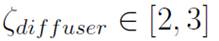 and the angle defining the slope (with respect the horizontal) of the diffuser
 must be in the interval
 with a preference for the lowest angles. Measurements of
 on the existing tunnel show that they are outside the established range, as well as the area ratio as it is shown in Table I.
Table I: Comparison between the suggested dimensions expected on standard design and the values measured on the existing wind tunnel

Stabilizer section. This section is included to correct the flow at the tunnel entrance by using a flow conditioner to stabilize the air currents. As occurs with the diffuser, the dimensions of the stabilizer section are set according to an area ratio
 , which should be in the Interval
 34, and the length L2 of stabilizer section is defined with the hydraulic diameter Dh = 2L2 = L1 of the stabilizer section 2. Table I lists the current values of the stabilizer section, as well as the corresponding expected ones by design.
Flow conditioner. The existing wind tunnel flow conditioner consists of a duct mesh with a circular cross-section of radius 0, 5 cm. Flow conditioners are essential to reduce the turbulence intensity and flow re-circulation, being the honeycomb mesh one of the most used in Wind tunnel designs 40. In principle, the structural rigidity of the mesh must be enough to withstand forces applied during operation without significant deformation 32), (33. For circular, square, or hexagonal flow conditioners with
 and equal tube areas, the loss coefficients K for each conditioner are 0, 30, 0, 25 and 0, 20. Here,
 is the hydraulic diameter of the cell, and L2 is the length of a cell that corresponds to the value of the length of the stabilization chamber. Approximately 150 honeycomb cells (for hexagonal flow conditioners) are defined per diameter for the stabilization chamber. A total of 25.000 cells needed in the flow conditioner is suggested. However, this can only be achieved in large-size wind tunnels 34.
Contraction. The contraction is a critical part in the design because it may have the largest impact on the flow quality in the test section 32),(33. Standard design suggests that
 must be set at 1, 25, where
 is the length of the contraction section (measured along the x-axis). Not only the dimensions of the contraction section, but also its shape plays an important role in the design, and there are simple but efficient analytic approaches to define the contraction curve. One of them is to define a polynomial whose coefficients are set depending on the dimensions of cross-sections in the stabilizer and the test section.
Contraction curve in two-dimensions The contraction is designed with a continuous and soft curve to minimize the negative effects when the cross section of the duct is decreased. If
 is a polynomial of degree 3 defining the contraction curve in two-dimensions (Fig. 2, left), then
 with
with
 real coefficients, which can be set depending on the length of the contraction section
 , the length H of the entrance, and the length h at the exit of the contraction. Additionally,
 is forced to pass through the middle point
 Coefficient
 s found by evaluating the function at zero,
 Since the function must have the middle point
 ,then
,then
 Similarly, we demand that / must have the point
 ;this is


Fig. 2: 2D Contraction curve. Cubic interpolation (left) Reflected curve (right). Black, red, and blue points are located at (0, H/2),(L/2,(H + h)/4) and (L, h/2) respectively. We used the following values L = 127cm, H = 100cm and h = 40cm on these plots.
These equations are not enough to find the polynomial coefficients. For this reason, it is necessary to impose another condition consisting on the annulment of the first derivative of
 at x = 0 or
 . Explicitly, the first derivative is
 . Hence,
 . They system can be written as
 , where
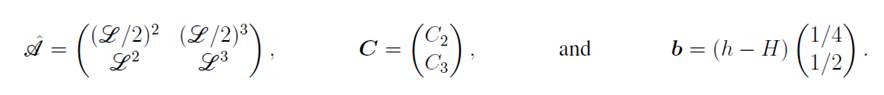
The solution of this 2 × 2 linear system is
 this is
 . It is also possible to use the condition Dxf(L) = 0 to find the coefficients, thus obtaining the same result for C1, C2 and C3. In sum, the contraction curve is f(x)
 with
with

 ,and
,and
 A plot of
 is shown in Fig. 2-(left). The other contraction curve is obtaining by a reflection with respect the x-axis as it is shown in Fig. 2- (right), where

It is possible to use the contraction curves on the plane
 in order to build the contraction section in the three-dimensional space. A curve in the space can be written as
 , where χ is the trajectory parameter. We define the contraction curves in the space as follows:

where
 are signs used to denote the fourth curves of the contraction section

 and
and
 which define its boundary. In Fig. 3 (left), we show the contraction section by setting
 , H and h with the same values used for bi-dimensional curves on Fig. 2. Finally, the wind tunnel including the proposed dimensions by design in Table I is shown in Fig. 3. To this aim, formulas in Eqs. (1) and (2) are employed to analytically define the parametric components of the curve, which can be introduced in 3D design software e.g. Solidworks. We would like to stress that there are other alternatives to choosing contraction curves, such as higher order polynomials. This topic is studied by author in Ref. 41.

Fig. 3: Modified wind tunnel. This plot is a modified version of the existing tunnel in Fig. 1 and includes suggested values for standard wind tunnels design.
There are other strategies to properly design the contraction curve of a wind tunnel 42)-(44 to reduce the wind tunnel losses and provide a high quality flow at the working section. For the case of low-speed wind tunnels, the contraction curve can be modeled by using polynomials of n − th order typically n = 3, 4, 5, or higher. A study regarding wind tunnels under the irrational incompressible model in Ref. (44 showed that contraction curves up to the 5th order without quadratic contribution provide good results at low velocities. There are also techniques concerning cubic spline curves, whose control points are properly set to enhance the the outflow at the end of the contraction section 42.
Governing equations
The dynamics of fluid flow are based on momentum, mass, and energy conservation laws. The set of mathematical expressions regarding these laws in fluids mechanics are known as Navier-Stokes equations. The Navier-Stokes momentum equation 45 for compressible fluid flow is

where v is the velocity field, P the pressure, µ the viscosity, g the gravity and ρ the density. The conservation of mass is given by the continuity equation

This work is limited to study the fluid in stationary conditions. For the continuity equation, this implies ∂tρ = 0. In general, the density into a wind tunnel is not uniform, since the air is a compressible fluid. However, it is possible to use the incompressibility approximation for lowspeed wind tunnels where the spatial variation of density is negligible. Under these conditions, the mass conservation law is

Thus the steady momentum equation (∂tv) takes the form of

The energy equation under steady conditions is

where
 is the vorticity, T is temperature, cv the specific heat capacity at constant volume, and κ is the thermal conductivity. This equation does not consider heating sources such as absorption or emission of radiation, but it considers heat transfer due to temperature gradients. In wind aerodynamics, it is generally reasonable to assume that air is a perfect gas, which implies that intermolecular forces are negligible. The equation of state of the ideal gas is P = ρRT, where R is the ideal gas constant. The energy of the ideal gas is U = CvT, with Cv being the heat capacity and the energy per unit of volume ρcvT. The system of Eqs. (3),(4),(5), and the state equation must be solved for the velocity components and the thermodynamic variables. This system of equations does not have a general analytical solution, and the problem is adressed with numerical methods. The system can be simplified depending on the regime of the flow. For instance, if the fluid flow in the tunnel is assumed to be laminar, the advective contributions (terms regarding the operator v · ∇) are small. If the fluid flow in the tunnel is laminar, the Mach number is small and the spatial variation of density negligible; then, it is possible to use the Bernoulli’s principle

if we move along a stream line with y being the elevation of the point above a reference plane. In fact, the Bernoulli’s principle is a consequence of the energy conservation along a single stream line of the fluid. Another approach to greatly simplify the problem is to model the tunnel as a bidimensional channel. Here, the continuity equation in two dimensions
 is satisfied by defining the components of velocity as
 , where
 is the two-dimensional stream function. This function can be obtained from the vorticity
 via the Poisson’s equation3

which reduces to the Laplace equation
 when fluid is considered irrotational. Modelling wind tunnels under a incopressible and irrotational assumptions simplifies a lot the equations of motion and it is possible to use potential flow solvers (see Ref. 44), but this approach is limited to low-speed wind tunnels.
Implementation of the numerical method
The Finite Difference FDM and Finite Element Methods FEM are standard numerical methods used for solving ordinary and partial differential equations. Even when there are software packages which enables to solve traditional problems in Computational Fluid Dynamics and Engineering 46)-(50, it is still useful to implement and programme the FEM including the meshing not only for fluid mechanics problems but also other problems in physics and engineering 51- 55) (56)-(58.
This section focuses on the application of the FEM in order to obtain numerically the stream function in the wind tunnel for an irrotational case, in oder words, when vorticity is negligible. A brief description of the interpolation functions, the discretization of the Laplace’s equation for the stream function and the definition of the two-dimensional mesh inside the tunnel will be shown.
3This equation is combined with the steady vorticity equation

which is obtained by taking the curl of Eq. (4). This is valid for low Mach numbers.
Global and local elements
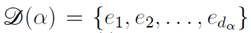
Let us consider a two-dimensional domain, where a mesh of elements has been defined with e = 1, . . . , M and M is the total number of elements. We shall use triangular elements in the plane, where N is the number of global elements and numbered with the index α = 1, . . . , N. Each triangular element (e) has three nodes located at the vertices of the triangle with positions x (e) m , where m = 1, 2, 3 as it is shown in Fig. 4. Two coordinate systems are then defined. The XY frame is a reference system used to define the global positions
 . On the other hand, the positions of the nodes in the xy frame will define the positions of those nodal points with respect to the center of each element. The geometrical center of each element, the centroid, is localized at
 (with respect to the XY frame) and is computed as an average of the local positions
 , where
 is the m-th nodal position of the elmement (e).

Fig. 4: Local elements employed in our simulations
Linear interpolation functions
Three local functions
 with m = 1, 2, 3 are defined on the nodes of each element. If they are linear, then
 , where a
 are coefficients. Local functions are shown Fig. 4-(right), and they are have the following property
 . The coefficients a (e) m are a constant
 59, and the coefficients
 can be computed with the local positions with respect to the centroid as follows:
 Similarly, the coefficients
 are
are
 the area of each element. The last determinant gives the area, assuming that local nodes are numbered in a counter-clock wise sense. Otherwise, this expression result in minus the area of the element. The node positions are computed as follows:
 This corresponds to a translation due to a change of reference frame. The global functions are defined as follows:
 ,
,
 is a boolean matrix that is 1 when the local node m of the element (e) is the global node Otherwise, it is zero.

Irrotational Flow
An approach to the laminar incrompressible flow at low velocities is to assume that vorticity is small everywhere. This implies that the stream function satisfies a Laplace’s equation

 where
where
 Defining S as the surface of the longitudinal section of the wind tunnel then
 ,
,
 with N the total gobal nodes in S.Then,

The last expression can be integrated by parts
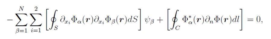
where
 is the normal derivative and the closed loop C is the boundary of S. Considering Dirichlet boundary conditions on C and defining M as the total number of inner nodes in S, then

with
 boundary points, and
 the values of the stream function on C, which defines the Dirichlet conditions.
Two-dimensional lattice: planar channel approximation
In this section a lattice construction in the internal geometry of the wind tunnel will be described. We start with a two-dimensional approximation of the tunnel, considering it as a two-dimensional channel. We define N0 as the number of boundary points. Procedure is a follows : we measured the positions of the boundary points of the tunnel. Later, all dimensions were rescaled with total length L of the tunnel, so the rescaled coordinates at the exit of the tunnel have an x-coordinate equal to the unit. We have defined four subsets of points
 and
and
 with the boundary points, where
 is the upper boundary,
 the lower boundary,
 the inlet, and
 the outlet.
The whole boundary is
 . A picture of the existing wind tunnel is shown in Fig. 1 (right). We have defined a piece-wise function
 by using the points of
 . Here,
 is built by joining the points boundary points
 with
with
 with straight lines. This is
 , where
 is a function of
 , which returns an integer number which labels the interval of piece-wise function

 Similarly, we used the same technique to define another piece-wise function
 corresponding to the lower boundary B2 of the wind tunnel. The functions f and g are used to define the inner points since these points satisfy
 if
if
 (0, 1), where S is the inner region. We wrote a short code in Mathematica to fill the region with points arranged in hexagonal lattice. Finally, a simple algothm in C++ was used to perform the Delaunay Triangulation of the points (Fig. 5).

Fig. 5: Meshing of the domain. Numbers in the boundary nodes corresponds to the stream function.
The velocity at the entrance
 is denoted as
 . We may use the following condition

 based on the mass conservation law to fix the velocity at the outlet
 . The inlet velocity is uniform, so the boundary condition on the stream function ψ at the entrance is

since
 . Similarly, the boundary condition on the stream function at the outlet is

The stream function in the upper boundary is set as follows:

and the stream function at the lower boundary is set as zero

Measurements
We have performed measurements at the entrance of the tunnel in order to find experimentally the distributions of the velocity, pressure and temperature. To this aim, we used a weather sensor including an anemometer, thermometer, and a barometer. The wind speed range of the sensor is
 with a speed resolution of
 and wind speed accuracy of ±3%. The barometer measures pressures from 150 to 1150 hPa (hecto pascals), with an accuracy of 1hPa and a resolution of 0, 03hPa. The temperature range of the device is
 of accuracy and / of resolution.
Measurements were performed at the center of the cells of a rectangular lattice defined at the entrance with dimensions
 with
with
 and
and
 , with
 and N = 12. The lenght of the square cell
 was chosen so that it fitted with the area of the anemometer. The center of the anemometer of the (i, j)-th measuerment was located at
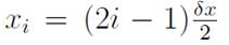 and
and
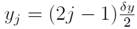 We performed 144 measurements of the inlet velocity, pressure, and temperature for the following values: 10, 27, and 53 Hz of angular velocity of the fan. The values of velocity, pressure and temperature for 10 Hz are shown in Table. II. Similar tables were built for 27 and 53 Hz.
Table II: Inlet parameters. Measurements on the entrance of the wind tunnel for 10Hz.
Although the frequency of the fan remained constant for each set of measurements, the flow speed at the inlet was not perfectly stationary and showed small variations, which ranged from 5 to 10% depending on the point where the measurement was made. In general, the fluctuations were slightly larger near the tunnel walls.
The pressure and temperature for 53 Hz are shown in Fig. 6. Small variations of pressure and temperature Fig. 6 are normal fluctuations due to the atmosphere. The average value of the barometric pressure
 and Temperature
 in the inlet are in Table. III for 10, 27 and 57 Hz. The averages are computed with the 144 measurements in the inlet, where σ and e are the standard deviation and relative errors, respectively. The mean values for pressure and temperature are independent of the fan frequency, since the the inlet is open to the atmosphere.
Table III: Mean values and error estimate of the inlet flow.


Fig. 6: Pressure (left) and temperture (right) at the inlet for 53 Hz.
In principle, it is expected to measure a uniform inlet velocity. However, it was observed variations in all velocity profiles for each fan frequency as shown in Fig. 7. These variations can be attributed to asymmetries in the diffuser, but also to the current design of the contraction section. In simulations, we take average of the inlet velocity as boundary condition. These average, along with their corresponding errors, are presented in Table. III.

Fig. 7: Left to Right. Inlet velocity profile for 10, 20, and 53 Hz .
Other sources of error on the fluid velocity measurements are the re-circulation and the fan noise. The flow generally tends to be turbulent at the fan outlet. Although, the wind tunnel studied is open, the entire structure is confined in a closed space4 . Therefore, the fluid from the fan outlet will enter the tunnel again at some point, and this will eventually affect the flow quality in the entire wind tunnel. The noise generated by the fan and the non-direct air re-circulation are factors difficult to control in open wind tunnels. Nevertheless, there are techniques for closed wind tunnels to reduce this type of noise, such as applying melamine foam on walls sections of the tunnel and the installation of acoustic baffle between walls of the tunnel 60.
Numerical simulations
We have to compute
 in order to solve the linear set of equations Eq. (6). By using the definition of the global functions, then
where
 is the set of elements associated to the global node
 , and
, and
 . Then, the local version of
 is
is

In practice, the computation of
 can be done strightfowardly from the boolean matrix since
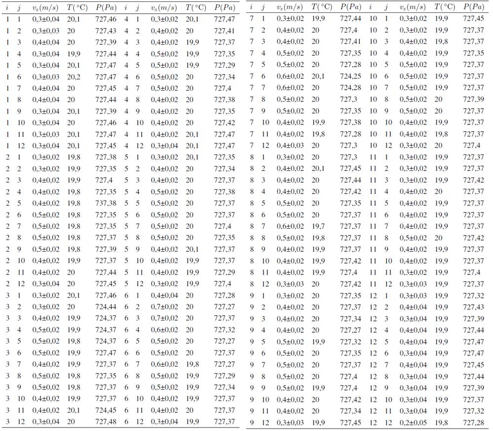
 for any elment (e) of the lattice. Since Eq. (7) has a lot of zero elements, then
 plays an important role because we may avoid the computational cost related to keep unnecessary zeros by computing the intersection between sets
 of different global nodes. Therefore,
 . We used the function Intersection of Wolfram Mathematica 9.0 61 to compute
 The local
 for linear interpolation functions is
 , and it can be evaluated straightforwardly from the parameters obtained in the Delaunay triangulation. Once the diffusion matrix is computed, the vector
 with the boundary conditions of the stream function is evaluated, and the system of equations given by Eq. (6) is solved. To this aim, it is standard to implement a Gradient Conjugated Method 62, however we simply decided to use the function NSolve of Mathematica. The numerical results of the stream function are shown in Fig. 8.

Fig. 8: Stream lines considering irrotational flow and two-dimensional approximation (left). Stream lines of the 3D system for 10 Hz without the irrationality condition.
The velocity field under the irrotational approximation is shown in Fig. 9 (left). This field is obtained from the stream function
 with the identity
 . To this aim, the values of the stream function on the elements nodes (see Fig. 5) are linearly interpolated to obtain a symbolic formula in Mathematica, and later that expression is derived.
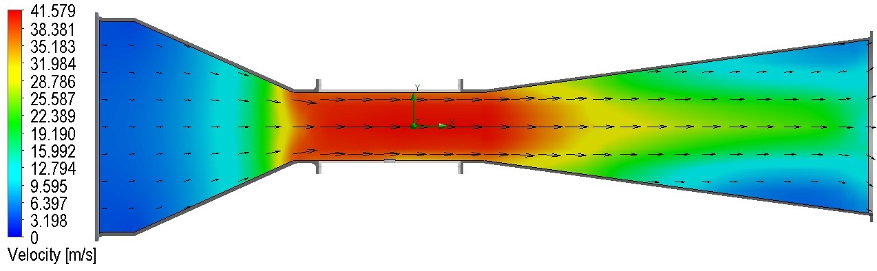
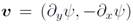
Fig. 9: Simulation under the irrotational assumption. Vector field (left) and velocity along the tunnel axis (right). The dashed line is the upper boundary of the wind tunnel.
The magnitude of the velocity along the x-axis under the irrotational approximation is shown in Fig. 9-right. The velocity value increases as the air flows along the contraction section. Later, it reaches its maximum velocity in the working section. In this section, the velocity profile has a plateau since the cross-section area is constant. Subsequently, the velocity decreases in the diffuser. This velocity profile is mainly a consequence of the restriction imposed by the incompressibility approximation given by the continuity equation
 . This leads to the condition
 constant with
 the cross-section area of the wind tunnel and
 the average x-velocity. Note that, in the bidimensionnal approximation of the wind tunnel, the cross-section only changes in one dimension, this is
 with
with
 a constant and
 the vertical separation between the bottom and top boundaries of the tunnel at a distance x. Hence, the continuity in the bidimensional approximation reads
 constant0 . Using this equation, the velocity in the working section can be obtained from the inlet velocity
 as follows:

since the velocity in the working section under this approximation is practically uniform

 . For the existing tunnel

 (Fig. 9, left), then the velocity ratio in the working section is
 as it is shown in Fig. 9 (right).
The data in Table IV was used to establish the boundary conditions of the numerical problem. The Stream function at the inlet
 is computed by integration of the inlet velocity components. Since the flow is under the incompressible approximation, then we used the continuity to establish the boundary conditions of the stream function at the outlet
 . The values of the stream function at
 and
and
 are kept constant, defining one of these constant as zero in the lower boundary
 .
.
Table IV: Average inlet flow

In our case, we used the default Solidworks solver for low Mach Numbers based on the Finite Volume Method, also known as Simpler Method. At the entrance of the wind tunnel, the pressure (in this case the atmospheric pressure) was specified. At the exit, the mass flow is used as boundary condition. The non-slip condition (zero speed) on the inner walls of the wind tunnel was specified. Regarding the measurements that were made experimentally from the velocity field at the entrance of the wind tunnel, then we know the mass flow in the input
 corresponding to the multiplication of the average speed by the entrance area
 , which is equivalent to compute the flux integral. The inlet flux can be computed by using the continuity equation
 0 with
 the cross-section area at another section in the tunnel e.g. the test section. The inlet flux is


The value of the velocity along the x-axis (middle points in the wind tunnel) is shown in Fig. 10. The solid red line in that figure corresponds to the evaluation of velocity according to the simulation, and the purple points are measurements of the velocity at points on the middle axis of the working section. The length of the error bars is estimated with
 , where ev is the percentage error of velocity in the inlet (see Table. III) and u is value registered by the anemometer at a point in the x-axis. In the working section, one can observe that the numerical and experimental data are in agreement. We do not provide measurements of the flow in the contraction and diffuser because it is difficult to place sensor in that section of the wind tunnel.

Fig. 10: Velocity along the tunnel axis for 10Hz. Red solid line and points corresponds to numerical simulation and measurements, respectively, in the working section (left). The gray dashed lines are represents the boundaries of the wind tunnel. The working section (right).
The result of these simulations for 10 Hz are shown in Figs. 8 (right) and 12. Even when the simulations are conducted with a compressible fluid, we observe that the density variation in the tunnel is negligible, so, for this frequency, the fluid incompressible, ∇ · v = 0. Similarly, the vorticity remains small in the tunnel, and velocity field is typical of a laminar flow with no vortices. This suggests that fluid flow in the tunnel for 10 Hz is practically irrational and incompressible. Therefore, the simulations of the stream function shown in Fig. 8 are still valid for low velocity operation of the tunnel, even though they were done assuming a channel in two-dimensions.
A comparison between the stream lines of Fig. 11 with the ones in Fig. 8 show that they are in agreement, except in the diffuser near the fan where the mass flux condition changes the stream lines.
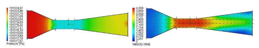
Fig. 11: Pressure distribution (left) and velocity field (right) for 10Hz.

Fig. 12: Density distribution (left) and vorticity (right) for 10 Hz.
We have also performed simulations on the geometry proposed in Fig. 3 with a better contraction curve and according to wind tunnel design criteria (see Figs.13 and 14). We can observe from the values of density, vorticity, and the velocity field that flow in the contraction and test sections can be approximated as irrotational and incompressible laminar flow. We would like to stress the fact that the solution of the Laplace equation for the stream function is laminar by default, because the incompressible and irrotational flow is a problem governed by a linear partial differential equation. On the other hand, the simulations performed with the fluid flow simulation package of Solidworks include the advective terms of the Navier-Stokes equations. Such terms are in part responsible of the difference between the the stream lines near the outlet of tunnel with and without the irrotational approximation (see Figs.8 and 11).

Fig. 13: Pressure (left) and velocity field (right) for

Fig. 14: Density (left) and vorticity (right) for 10 Hz.

Fig. 15: Velocity field. 27 Hz (left) and 53 Hz (right).
The results we found for 27 and 53Hz are similar to the ones presented for 10 Hz but with velocity values in larger range (see Fig. 15). However, we do not rule out the meshes used in these simulations, along with the Simpler Method, could not sufficiently fine to capture the contributions of the non-linear terms of the equations correctly. Previous experimental studies 63 they used Reynolds numbers of the order of
 in order to find the thickness value of the layer limit for a NACA23012 profile, where it was assumed that flow behaved laminarly because its Reynolds number does not exceed the value of
 In this work, the Reynolds number is in the range of
 , corresponding to the frequency range of the fan. A comparison of the Reynolds numbers calculated in this document with those provided in 63 suggests that the flow that would be observed in the wind tunnel studied here is in the laminar regime.
The distribution of vorticity in the working section is shown shown in Fig. 16. One of the advantages of modifying the contraction section and the diffuser corresponds to an improvement in the quality of the flow in the working section. If a comparison of the vorticity of the existing tunnel (see Fig. 1) and its modified version (see Fig. 3) is made, then a less intense vorticity distribution can be observed in the test section of the modified wind tunnel.
Another factor that can affect the production of vorticity inside the test chamber concerns its design because it has a lid on its bottom (Fig. 10, right). This is used to cover a hole where a metal lab bracket can be installed to eventually hold a test object. For low velocities, the impact of the lid is small, and it can be removed with a better design on the contraction section, but the lid can favor production of vorticity as the velocity increases. This occurs at 53 Hz in Fig. 16 (right).

Fig. 16: Vorticity in the working section. The values of vorticity are presented in s−. Vorticity in the working section of the existing tunnel (left) and the modified tunnel (center) for 10 Hz. Vorticity at 53 Hz (right).
Conclusión
In this study, numerical simulations and experimental measurements were carried out in order to characterize the flow inside a low-speed wind tunnel. One of the implemented strategies modeled the tunnel as a two-dimensional system, with a incompressible and irrotational fluid flow. Under these assumptions, the flow is potential, and it can described by the stream function. In the second approach, we removed the irrationality and incompressibility conditions, and simulations were performed in three-dimensions. We found that the stream lines into the wind tunnel were quite similar, regardless of the approach for low flux velocity in the laminar regime, as it was shown in Fig. 9. This is useful since the fluid flow with irrotational and incompressibility conditions numerically is is easier to simulate numerically and computationally less expensive than simulations of fluid flow without these assumptions.
Simulations without incompressibility conditions showed that density variations into the tunnel were small. This was observed in the density distribution of the real and modified wind tunnel shown in Figs. 12 and 14. In those figures, there is no density changes up to the 4th significant digit, which represents a percentage change smaller than 0, 05%. Therefore, the velocity field into the studied low-speed wind tunnel is practically divergenceless, even though air is a compressible fluid.
Asymmetries on the wind tunnel walls, fan noise, re-circulation, and the type of tunnel design can affect the quality of the flow. Spatial variations measured in the inlet of the wind tunnel can be a combination of all these factors. These problems, attributed mainly to the design of the device, also affected the measurements in the working section, even when they seemed to be in agreement with numerical simulations of the velocity on the x-axis. In this study, we proposed changes on the contraction and diffuser with the aim of enchancing the flow quality. Changes in the contraction with third-order polynomial curves resulted in an important reduction of vorticity in the working section of the modified tunnel with respect the original device as it was shown in Fig. 16. This reduction in the intensity of vorticity is not due to a decrease in the magnitude of velocity, since both contraction sections (modified and original) connect the same inlet and outlet areas (Fig. 12 and 14) as well as the fact that air behaves as incompressible in the tunnel.
As a future work, it would be interesting to model the inner fluid flow of the wind tunnel by using numeric-analytic techniques such as collocation methods 64 used for micro channels or mesh-less methods as the one described in 63.
Acknowledgements
Acknowledgment
This work was supported by the Research Vice-Principalship of Universidad ECCI.
References
Licencia
Derechos de autor 2022 Andrés Lara, Jonathan Toledo, Robert Paul Salazar Romero

Esta obra está bajo una licencia internacional Creative Commons Atribución-NoComercial-CompartirIgual 4.0.
![]()
A partir de la edición del V23N3 del año 2018 hacia adelante, se cambia la Licencia Creative Commons “Atribución—No Comercial – Sin Obra Derivada” a la siguiente:
Atribución - No Comercial – Compartir igual: esta licencia permite a otros distribuir, remezclar, retocar, y crear a partir de tu obra de modo no comercial, siempre y cuando te den crédito y licencien sus nuevas creaciones bajo las mismas condiciones.

2.jpg)