DOI:
https://doi.org/10.14483/23448393.19252Published:
2022-08-12Issue:
Vol. 27 No. 3 (2022): September-DecemberSection:
Electrical and Electronic EngineeringFlujo de potencia en redes de distribución eléctrica trifásicas no equilibradas utilizando Matlab: Teoría, análisis y simulación cuasi-dinámica
Power Flow in Unbalanced Three-Phase Power Distribution Networks Using Matlab: Theory, analysis, and quasi-dynamic simulation
Keywords:
load flow, Newton's method, Backward-forward algorithm, power flow, quasi-dynamic simulation (en).Keywords:
flujo de carga, método de Newton, algoritmo de barrido iterative, flujo de potencia, simulación cuasi-dinámica (es).Downloads
References
F. Milano, Power system modelling and scripting. Berlin, Heidelberg: Springer Berlin Heidelberg, 2010. DOI: https://doi.org/10.1007/978-3-642-13669-6
G. W. Stagg and A. H. El-Abiad, Computer methods in power systems analysis, vol. 4. Deli, India: McGraw
Hill, 1988.
B. Stott and O. Alsac, “Fast decoupled load flow,” IEEE Transactions on Power Apparatus and Systems,
vol. PAS-93, pp. 859–869, May 1974. DOI: https://doi.org/10.1109/TPAS.1974.293985
R. K. Portelinha, C. C. Durce, O. L. Tortelli, and E. M. Lourenc ̧o, “Fast-decoupled power flow method for inte-
grated analysis of transmission and distribution systems,” Electric Power Systems Research, vol. 196, p. 107215,
How to Cite
APA
ACM
ACS
ABNT
Chicago
Harvard
IEEE
MLA
Turabian
Vancouver
Download Citation
Recibido: 2 de abril de 2022; Aceptado: 23 de mayo de 2022
Abstract
Context:
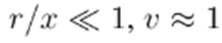
The power flow is a classical problem for analyzing and operating power distribution networks. It is a challenging problem due to a large number of nodes, the high r/x ratio -typical in low voltage networks- and the unbalanced nature of the load.
Method:
This paper review four methods for power flow analysis, namely: the conventional Newton’s method, Newton’s method in a complex domain, the fixed-point algorithm using Y bus representation, and the backward-forward sweep algorithm. It is well-known that Newton’s method has quadratic convergence, whereas the backward-forward sweep algorithm has linear convergence. However, the formal analysis of this convergence rate is less known in the engineering literature. Thus, the convergence of these methods is presented in theory and practice.
Results:
A set of simulations in the IEEE 900 node test system is presented. This system is large enough to demonstrate the performance of each algorithm. In addition, a Matlab toolbox is presented for making numerical simulations both for the static case and for quasi-dynamic simulations.
Conclusions:
Fixed point algorithms were faster than Newton’s methods. However, the latter required less number of iterations.
Keywords:
load flow, Newton’s method, Backward-forward algorithm, power flow, quasi-dynamic simulation..Resumen
Contexto:
El flujo de potencia es un problema clásico para la operación de redes de distribución de energía. Es un problema desafiante debido a la gran cantidad de nodos, la alta relación r/x típica de las redes de baja tensión y la naturaleza desequilibrada de la carga.
Métodos:
Este documento revisa cuatro métodos para el análisis de flujo de potencia, a saber: el método de Newton convencional, el método de Newton en un dominio complejo, el algoritmo de punto fijo que utiliza la representación de admitancia nodal (Y bus) y el algoritmo de barrido hacia atrás y hacia adelante. Se presenta la convergencia de estos métodos en teoría y práctica. Es bien sabido que el método de Newton tiene convergencia cuadrática, mientras que el algoritmo de barrido hacia atrás y adelante tiene convergencia lineal. Sin embargo, el análisis formal de esta tasa de convergencia es menos conocido en la literatura de ingeniería.
Resultados:
se desarrolla una caja de herramientas de Matlab para realizar simulaciones numéricas tanto en el caso estático como en una simulacion cuasi-dinámica usando el sistema de pruebe IEEE de 900 nodos.
Conclusiones:
Los algoritmos de punto fijo resultaron mas rapidos. No obstante, los algoritmos basados en Newton requirieron menor número de iteraciones.
Palabras clave:
flujo de carga, metodo de Newton, algoritmo de barrido iterative, flujo de potencia, simulación cuasi-dinámica..Introduction
Power flow is a standard method for analyzing and operating power systems both at high voltage levels and in power distribution networks. It takes nodal power information and returns the system’s state, which is usually represented by nodal voltages. The problem consists of a large set of highly nonlinear algebraic equations that requires efficient numerical methods to be solved in practice 1. Newton’s method is undoubtedly the most common approach for high power applications. It searches for the solution using successive linear approximations via Taylor’s expansions. These approximations require calculating a Jacobian matrix in each iteration. However, calculating this Jacobian matrix and solving the corresponding linear system may be computationally expensive. Therefore, particular approximations have been proposed according to the type of network. For example, in high-voltage power transmission networks, the resistance value tends to be lower than the inductance of transmission lines, so the Jacobian matrix can be reduced to a constant matrix directly related to the imaginary part of the nodal admittance matrix. This matrix can be efficiently factorized using lower-upper decomposition or Cholesky’s factorization in order to solve the linear system quickly 2 for a complete review of these methods). These quasi-Newton methods are known as decoupled and fast-decoupled Newton’s methods 3. The most simplified version of the problem consists of a linear system that neglects voltage variations. This method is called DC-load flow due to the analogy to the problem of finding voltages in a DC network 4. Unfortunately, that kind of approximation is not valid in power distribution networks, and the entire Jacobian must therefore be constructed in each iteration 4.
Newton’s method (without any approximation of the Jacobian matrix) has quadratic convergence, -even in power distribution networks- when initialized close to the solution. This property has been analyzed mainly in the context of DC grids 5, although it can be extended to AC networks. This method can also be defined in the complex domain using Wirtinger’s derivatives 6. However, the algorithm is still time-consuming in both cases due to the construction and inversion of the Jacobian matrix, which is why Jacobian-free algorithms are used in power distribution networks. These ad-hoc algorithms include the backward-forward sweep method and the current injection method 7.
The backward/forward sweep algorithm is the standard in power distribution networks . This algorithm considers power distribution networks as radial, and it executes a two-step iteration based on Kirchhoff’s laws: first, line currents are calculated in a backward sweep, i.e., starting from the last node in the direction to the substation; then, voltages are calculated in a forward sweep, i.e., from the substation to the final user. This simple method has been used in academic and commercial software due to its flexibility and efficiency 9. It allows solving single-phase and three-phase unbalanced systems. Moreover, it may be easily modified to include voltage regulators and other compensation components 10.
A less known aspect of the backward/forward sweep algorithm is its theoretical analysis 11. The algorithm is, in essence, a fixed-point iteration that guarantees a linear convergence (in contradistinction to the quadratic convergence of Newton’s method). This algorithm can be represented in matrix form, thus allowing for a simple implementation in interpreted languages such as Matlab or Python. Moreover, a matrix representation allows for a straightforward analysis 12.
On the other hand, modern analysis in power distribution networks requires simulations in a time window while considering variations in generation and load. This type of simulation, known as quasi-dynamic time series analysis, requires the evaluation of thousands of power flow scenarios, so efficient algorithms are required today more than ever 13.
Despite being a classic problem, power flow is still under research 14, where neural networks 15 and distributed implementations are two areas of constant development 16, 17. Its implementation in large power systems is also a challenge that is constantly studied 18, as well as its practical implementation 18. Although using artificial intelligence techniques can be justified in some specific contexts, the scientific community has heavily criticized its abuse [19]. A classic approach is always preferable since it starts from understanding the physical phenomenon and ensures general mathematical properties that cannot be assured by means of artificial intelligence. Therefore, it is important to review and analyze classic problems and their solutions.
This paper analyzes four power flow algorithms for power distribution networks, namely the conventional Newton’s method, the Newton’s method in a complex domain, the fixed-point algorithm using Ybus representation, and, the backward-forward sweep algorithm. Contributions are twofold: first, the algorithms are presented in general form, and their convergence is analyzed in theory and practice; and second, a toolbox in Matlab is developed to compare each formulations. To the best of the author’s knowledge, there is no other toolbox in Matlab that deals with unbalanced power distribution networks as presented herein.
The rest of this paper is organized as follows: Section 2 presents the basic formulation of the power flow problem for three-phase unbalanced systems; Section 3 presents Newton’s method, both in its real formulation and in the complex domain; after that, the fixed-point algorithm and the backward-forward sweep method are presented in Section 4; Section 5 provides a review of the fundamental theoretical analysis of these algorithms; and Section 6 shows numerical experiments using the IEEE 900-node test system. The paper ends with conclusions in Section 7 and a brief appendix about the Matlab implementation.
Problem formulation
A power distribution network is represented by an oriented graph
 , with
 being the set of nodes and
 the set of branches. The size of
 is
is
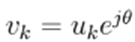
 . Uppercase letters represent vectors and matrices, while lowercase letters represent single variables or vector/matrix entries. Thus, the nodal voltage is given by
 and the nodal power is given by
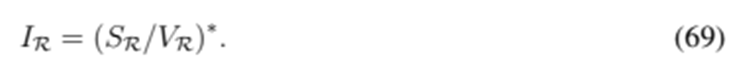
 . All variables are considered to be complex hereafter unless otherwise specified. The complex conjugate of x is represented by x∗. This operation is only the conjugate without transposing when applied to a matrix . With a slight abuse of notation, X/Y represents the element-wise array division between vectors X and Y of the same size.
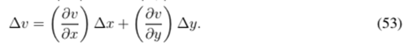
Nodal voltages and nodal currents are related by the following matrix equation:
where Y is the nodal admittance matrix  . Each entry of this matrix is constructed as follows:
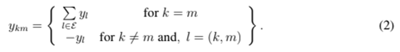
This equation indicates, in simple terms, that the entries in the diagonal collect the admittance of all the lines connected to a node, and that the off-diagonal terms collect the negative of the corresponding line admittance. Another way to construct the nodal admittance matrix is presented below:
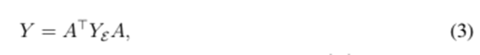
where A is the node-to-branch incidence matrix associated to  and
and 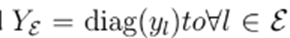 The nodal power is represented in terms of the nodal current, as given in Eq. (4):
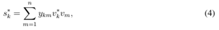
where  indicates the complex conjugate of
  This equation can be split into real and imaginary parts, as given below:
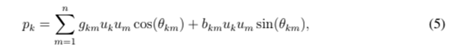
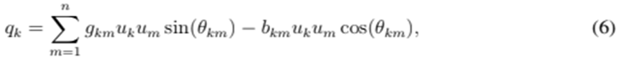
where
 and
and
 , with
 and
and
 being real variables. The power flow consists of finding
 given the value of
 at all nodes except the substation, as the voltage of that node is already known. The problem is clearly nonlinear and highly complex, so numerical methods are required to find a solution. Note that Eqs. (5) and (6) are completely equivalent to (4), although the latter is undoubtedly a more compact representation. Eq. (4) is known as the complex representation of the power flow, whereas (5)-(6) is a real representation thereof.
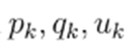
On the other hand, power distribution networks are unbalanced, and hence this model must be extended accordingly. Thus, each node in the graph represents three nodes in the system, which are labeled as A, B, and C, as depicted in Fig. 1. Likewise, each branch represents a three-phase line section with its corresponding 3 X 3 impedance matrix. The algebraic structure of the problem is the same for three-phase systems; only the size is increased.
Figure 1: Example of a three-phase line for modeling three-phase unbalanced power distribution networks
The three-phase nodal admittance matrix
 is constructed in the same way as in Eq.(2), but, in this case,
 is a 3 X 3 block matrix. There is also an equivalent formulation using the node-to-branch incidence matrix, as given in Eq. (7).

where I3 represents the identity matrix of size 3, and
 is the Kronecker’s product. Both formulations return a matrix in which entries 1 to n correspond to phase A, entries n + 1 to 2n correspond to phase B, and entries 2n + 1 to 3n correspond to phase C. From now on, the three-phase case is considered in this article since it is the most general.
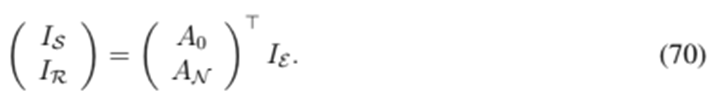
The substation consists of three nodes corresponding to each phase. These nodes are represented by the set
 . The remaining nodes are
 . Then, the nodal voltages are divided into two sets, namely
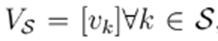 , and
, and
 . The same applies to currents
 nodal powers
 and nodal admittance matrix
 .
.
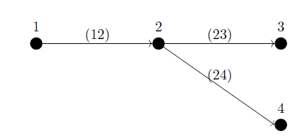
Power distribution networks are usually radial. Therefore, their graphs have a particular structure known as tree, in which any two vertices are connected by exactly one path. As a consequence of that, each branch has a unique arriving node, as exemplified in Fig. 2.
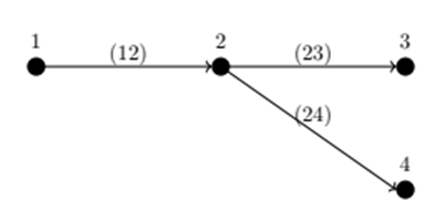
A tree structure is vital for the backward-forward sweep algorithm, as presented in Section ??. This property allows for the creation of an unambiguous map between branch currents and the set of nodal voltages. This map has two consequences, one theoretical and one practical. From a theoretical point of view, the submatrix Y is non-singular if the graph is connected, This property is used by the fixed-point algorithm. From a practical standpoint, this map allows for efficient storage in the same array in the backward-forward sweep algorithm. Along this paper, it is supposed that the branches are sorted from the substation to the final user and the currents in the graph are oriented accordingly (20 for a graph ordering method).
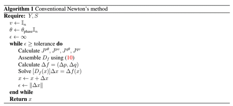
Newton’s methods
Conventional Newton’s method in the real domain
Newton’s method is a classic algorithm for solving optimization problems and systems of nonlinear algebraic equations such as the power flow problem. It approaches the solution by successive linear approximations of the non-linear equations, as depicted in Fig. 3. The method departs from an initial guess X 0 , where the non-linear equation is approximated linearly. A new point X 1 is calculated, and the function is again approximated to a linear form. The process continues until an acceptable solution is found 21.
Each iteration of Newton’s method has two key steps: first, the derivative of the function is calculated, and then, the new operation point is evaluated. The following expressions show the process:


In the power flow problem, the function f is usually defined by separating the power flow equations into real and imaginary parts, i.e., (5)-(6). The vector of state variable is  , and
, and  is the Jacobian matrix given by Eq. (10),
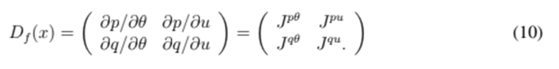
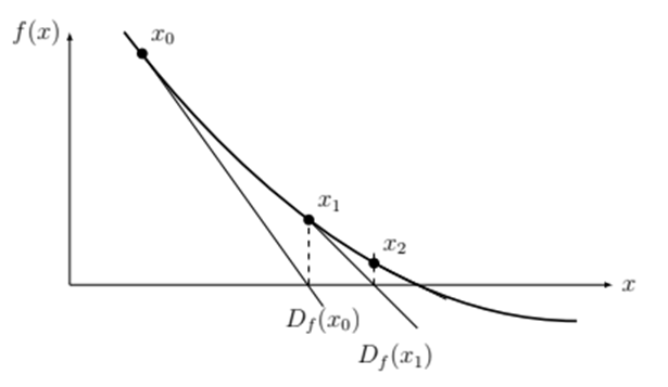
Figure 3: Simple representation of Newton’s method
The Jacobian is a block matrix that requires separately considering diagonal and off-diagonal entries. The diagonal entries are given below:


and the non-diagonal terms are given by the following expressions:


Algorithm 1 summarizes the main steps of the conventional Newton’s method applied to power distribution networks.
Newton’s method is computationally expensive since
 has to be calculated in each iteration. In addition, it is necessary to calculate the step either by inverting
 or by solving the linear system (8). Both options are time-consuming. In high-voltage power systems, it is possible to simplify the problem by making two main approximations: first, the pθ problem is separated from that of qu based on the fact that
 and
and
 ; second, the sub-matrices
 and
and
 are considered to be constant since
 , and
, and
 ≪ 1. Unfortunately, these approximations are not valid in power distribution networks, and this method is therefore rarely used in this type of networks.
The method can be easily extended to three-phase unbalanced systems, considering initializing the voltages to 1 pu with the proper phase
(i.e., 0 for phase
 for phase B, and
 for phase C). The mathematical properties of the algorithm are the same in the single-phase and the three-phase cases.
Newton’s method in the complex domain
The complex representation of the power flow is undoubtedly more compact than the real representation. Therefore, Newton’s method is expected to be equally compact in the complex domain.
The following definition is required to obtain the linearization:
Definition 3.1. Given a complex function
 with
with
 , the Wirtinger’s derivative and its conjugate are defined as follows:


Definition 3.2. A function
 is holomorphic if its Wirtinger derivatives exist and
 .
.
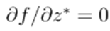
Holomorphic functions are complex and differentiable. This one infinitely differentiable and locally equal to its own Taylor series. This also means that the following limit can be taken from any direction (see Fig. 4):

Another way to identify holomorphic functions is via the Cauchy-Riemann equations presented below:
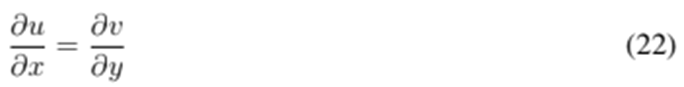
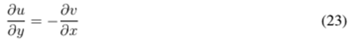
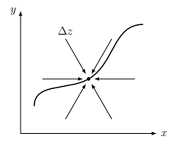
Figure 4: Possible directions in which limit (21) can be taken in the complex domain
Thus, if f is holomorphic, then Wirtinger’s derivative is equal to the standard complex derivative. Unfortunately, the power flow equations are non-holomorphic, so a linearization must consider the effect of both the variable and its conjugate.
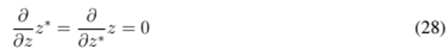
In general, Wirtinger’s derivatives apply the common rules of differentiation known from realvalued analysis concerning the sum, product, and composition of functions, namely:
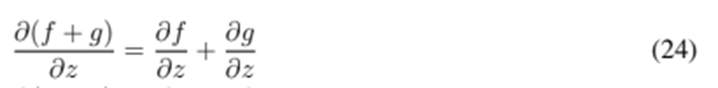

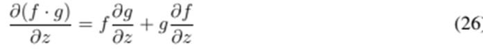
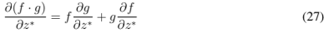
Operations are similar to those in partial derivatives, so
 can be regarded as a constant when computing the derivative with respect to z and vice versa:
A complex linear approximation of f can be obtained using these simple definitions, as shown below:
This approximation behaves like the Jacobian matrix when
 , and it can be applied sequentially by using the iteration
 . The complex linearization of Eq. (4) is presented below:
This equation can be written in matrix form, thus obtaining the following affine equation:

where JA and JB are the complex square matrices defined below:


Note that Eq. (31) depends of
 and
and
 . Therefore, it is not as simple as a conventional linear system. First, the complex conjugate is calculated:

Then,
 is represented as function of
 :
:
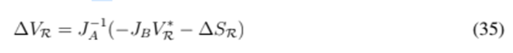
Finally, (35) is replaced into (34), and
 is cleared:

This equation may be efficiently solved by defining auxiliary matrices M1 and M2, as follows:


In this way, only one inverse is directly calculated (i.e., the inverse of
 ), and this inverse is constant. Newton’s method in the complex domain is presented in Algorithm 2. The method can be extended to three-phase unbalanced systems by considering the three-phase admittance matrix and a proper initialization of the nodal voltages, taking the corresponding phase into account. Note that the method has a simple and clean code that enables to adapt the script to new problems. This is the main advantage of complex representation.

Fixed-point methods
Direct formulation
Another widely used method for solving nonlinear equation systems is transforming the problem into a fixed point. The Gauss-Seidel method is an excellent example of this approach. This method is widely used for solving systems of linear equations, and it has also been used for solving power flow equations by employing the following iteration:
This method is important for historical reasons, as it was one of the first approaches for solving the power flow problem. However, it suffers from convergence issues, and hence it is rarely used in practice. Nevertheless, it is the origin of other fixed-point algorithms that are more useful in practice. Before presenting these algorithms, the concept of fixed point should be formally defined.
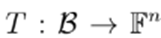
Definition 4.1 (Fixed point). Let
 be any space and T a map of
 into
. A point
into
. A point
 is called a fixed point for T if
 .
.
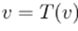
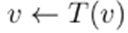
Fixed point-theory allows solving the equation
 by searching for a fixed point of

 . In some cases, this fixed point can be calculated by iteratively applying
 . The method converges if the map T is a contraction as explained in Section 5.
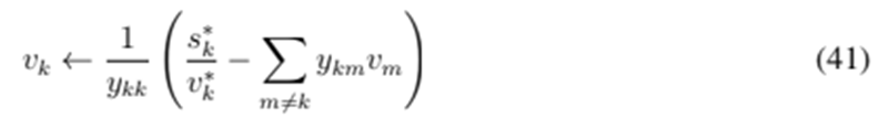
It is straightforward to find a map T in power distribution networks. First, the nodal power is represented in matrix form, separating the current in the slack from the remaining nodes, as given below:
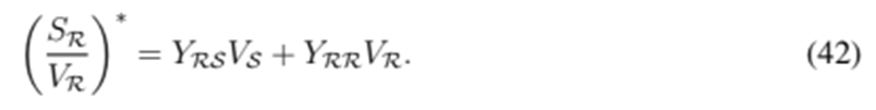
Second, the nodal voltage is cleared as follows:
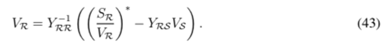
Finally, a map T is obtained:
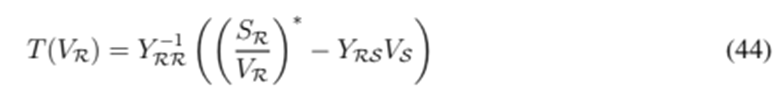
Note that the inverse of YRR only needs to be calculated once. Another option is to calculate the result of the map without explicitly calculating this inverse. The matrix
 is sparse, so this option may be more efficient. Algorithm 3 summarizes the main steps of this fixed-point method. Note the simplicity of the algorithm.
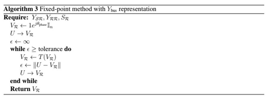
The method is the same for single and three-phase networks. As in the previous cases, the admittance matrix is three-phase, and the voltages’ angles need to be initialized properly. Note that the method does not impose any constraint related to the radiality of the grid. The method can be easily extended to consider ZIP loads and renewable power (this aspect is beyond the objectives of this review).
Backward-forward sweep algorithm
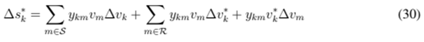
Another fixed-point algorithm can be obtained by using some particular characteristics of power distribution networks. The strategy consists of making use of the tree structures of the graph associated with this type of network. This structure allows solving the power flow problem by applying Kirchoff’s circuit laws in three steps: first, the nodal current is calculated from the nodal power and voltage; second, Kirchoff’s current law is applied from the last user back to the main substation in a backward sweep; third, Kirchoff’s voltage law is applied from the substation to the last user in a forward sweep iteration. The method is known as the backward/forward sweep algorithm for obvious reasons. Algorithm 4 represents the pseudo-code for this method. All nodes are expected to be ordered from the substation to the final users.
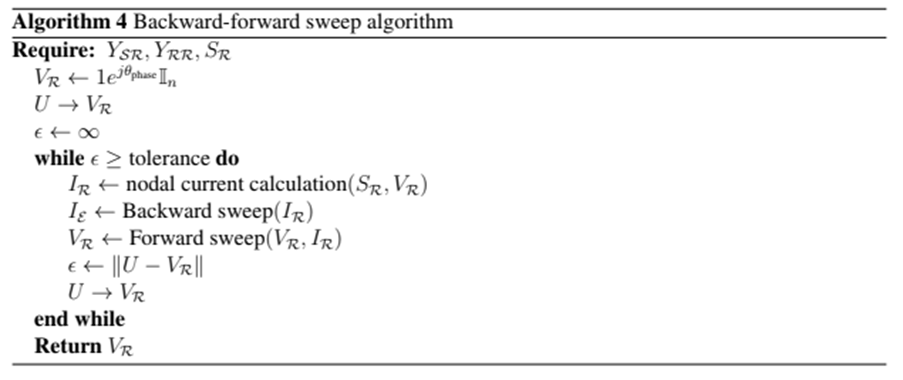
Each of the steps are explained below with the help of the graph given in Fig. 2. First, the nodal current is calculated for each node except the slack node. The following expression is used:
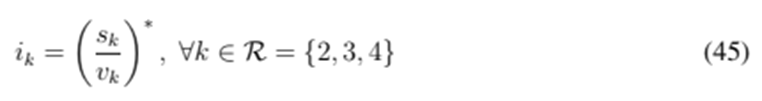
Then, the branch currents
 are calculated using nodal currents
 . This step is known as backward sweep. The calculations for the graph depicted in Fig. 2 are given below:


An important detail of implementation: branch currents are stored in the same array as nodal currents since there is only one receiving node for each branch. Thus,
 now stores
 ,
,
 stores
 and
and
 stores
 . Finally, the new voltages are calculated in a forward sweep, namely:


The main advantage of this method is that no matrix needs to be inverted -not even the nodal admittance matrix. In addition, the method can be easily extended to the three-phase case, and it constitutes a fixed point since the nodal voltage is calculated from the nodal voltages in each iteration 22. The only difference is that the map is not explicitly defined 23. The next section presents a formal analysis of this and the previous methods.
Equivalences, convergence, and analysis
This section analyzes the equivalence between the two pairs of algorithms presented in the last section. It also presents results related to the convergence as well as insights about its practical implementation. Four methods have been presented at this point: Newton’s method, complex sequential linearization, the fixed-point method with Ybus representation, and the backward-forward sweep algorithm. The first two algorithms are based on linear approximations of the non-linear equations, whereas the last algorithms are based on fixed-point theory. Although each algorithm requires a different implementation, they have some equivalences from the theoretical point of view.
Definition 5.1. Consider two power flow algorithms A and B, where the voltage in iteration k of A is
 and the voltage in iteration k of B is
 . A and B are behaviorally equivalent if
  , where ε is a rounding error.
It is easy to obtain the equivalence between the conventional Newton’s method and Newton’s method in complex domain by using the following result:
Lemma 1. Sequential complex linearization is behaviorally equivalent to the linearization used by Newton’s method.
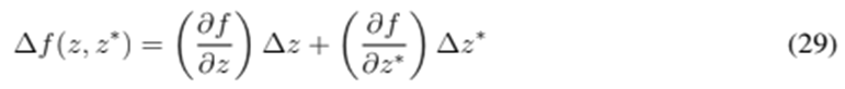
Proof. Replace z = x+jy and f = (u, v) in Eq. (29) and note that it is equivalent to the following linearization’s real and imaginary parts:
This is clearly the same linearization obtained for Newton’s method applied to the vector function f = (u, v).
Algorithms 1 and 2 are just two representations of the same linearization. Hence, their convergence properties are the same. However, the convergence of two equivalent power flow algorithms does not imply the same time calculation. Two algorithms can have the same convergence plot but different time calculations. Simple aspects such as the programming language and the way the information is stored may drastically change the performance of the algorithm. This aspect is analyzed in the results section.
On the other hand, Newton’s method has a well-defined convergence behavior, which is given by the Kantorovich theorem (24):
Theorem 1. (Kantorovich theorem in
 ) Let
) Let
 be a point in
and
be a point in
and
 a differentiable map with an invertible derivative
 . Define


if the derivative
satisfies the Lipschitz condition,

and if the inequality
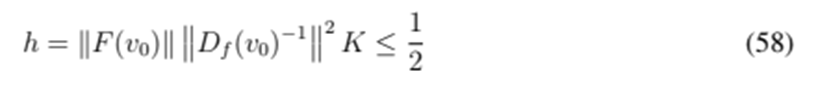
is satisfied, then the equation F(v) = 0 has a unique solution in
 , and Newton’s methods converges to it with Newton’s step 9 and an initial condition
 . Moreover, if
 , the order of convergence is at least quadratic.
This result is well-known in the scientific literature 25. However, for the sake of completeness, a sketch of proof is presented below. This proof is built upon the work of 26.
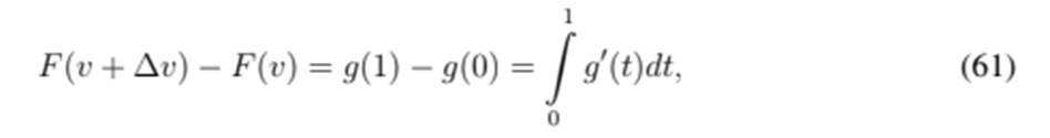
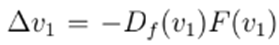
Proof. Let us define
 . Then, by replacing I = Df
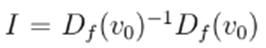 and bythe Lipschitz condition of
 , following is obtained:

but
 and, due to condition (58),
 . Therefore, the Banach Lemma can be used, which guarantees the existence of the inverse of (I − A) and gives boundaries as follows:

On the other hand, let us define a function
 then,
then,

 , and hence
that is,
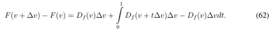
By the Lipschitz condition of
 , the following is obtained:

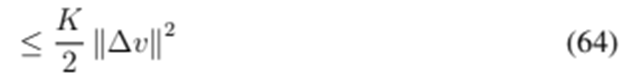
since
 in each iteration. Then,
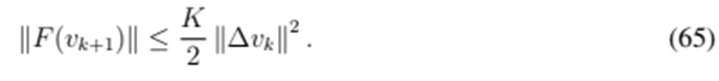
Finally, let us analyze the step
 , which, by applying (60), (65), and (58), yields the following:


By applying the same argument to the next iterations, it can be concluded that there is a contraction of
 and F(v).
The Kantorovich theorem ensures quadratic convergence when the initial approximations are such that conditions (54) to (56) hold. However, these conditions are quite severe and may not be fulfilled by a given scenario. Therefore, it is very important to select a suitable initial condition. In the case of three-phase unbalanced systems, the initial conditions are
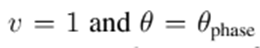 according to the phase. When all conditions are fulfilled, the algorithm converges to the power flow solution, and this solution is unique.
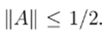
The uniqueness of the solution is an essential aspect of this type of analysis. The convergence of an algorithm may be evaluated through a sequence of numerical simulations. However, there can always be doubt about whether this is the only possible solution. Theorems like Theorem 1 ensure that there are no other possible solutions in the region
 . There might be other solutions in other regions, but the solution in
is unique. It is usual that this other solution lacks physical meaning by considering, for example, voltages with negative magnitude and angles higher than
. There might be other solutions in other regions, but the solution in
is unique. It is usual that this other solution lacks physical meaning by considering, for example, voltages with negative magnitude and angles higher than
 Understanding the physics of the problem is important to use theoretical results correctly.
There are also convergence and uniqueness conditions for fixed-point algorithms, which are analyzed below:
Lemma 2. The fixed-point method with Ybus representation is behaviorally equivalent to the backward-forward sweep algorithm.
Proof. The first step of the backward-forward sweep algorithm consists of calculating nodal currents. This step is represented in matrix form as given below:
Nodal currents are related to branch currents by the incidence matrix given below:
The sub-matrix
 is non-singular, since the grid is radial (i.e., the graph is a connected tree). Therefore, it is possible to obtain branch currents from nodal currents as
 . This step corresponds to the backward current sweep.
On the other hand, branch voltages are related to nodal voltages as follows:

and to branch currents by the Ohm’s law, namely

This calculation corresponds to the forward voltage sweep. By collecting all the previous expressions, the following fixed-point is obtained:
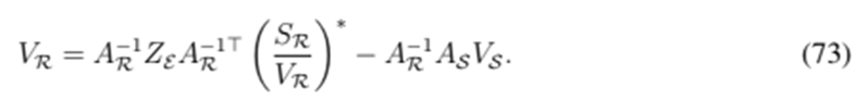
It is straightforward to demonstrate the following equivalences:


Hence, Eq. (73) is equivalent to Eq. (43).
Considering that Algorithms 3 and 4 are equivalent, their convergence can be analyzed.
Definition 5.2. Let
 be a closed ball of
 , and let
 . Then,T is said to be a contraction mapping if there is a
 such that
 , with
 .
.
Theorem 2. If T is a contraction mapping, then there is a unique
 satisfying
 , whichcan be obtained by applying iteration
 starting from an initial point in

Proof. The contraction mapping theorem is general for any Banach space, but we are interested in
 be a contraction mapping in a closed ball
 . Considering two points u, v ∈
 , the following is obtained:


Rearranging the expression yields the following result:

Clearly, if u = T(u) and v = T(v), then
 . Since a norm is always positive except inzero, then necessarily u = v, which means that the fixed point is unique.Now, let us define a sequence
 by the iteration
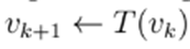 . Then, it follows that

Therefore,
 is a Cauchy sequence. Since Rnis complete, then
converges to a fixed
is a Cauchy sequence. Since Rnis complete, then
converges to a fixed
 . More details about this theorem can be found in 27 and 28.
Contraction mapping theory is important because it guarantees the convergence of the fixed-point algorithm. In addition, it ensures the uniqueness of the solution, just as in Newton’s method. However, the convergence rate given by Eq. (80) is linear, while the convergence rate of Newton’s method is quadratic. These convergence properties are numerically evaluated in the next section.
Results
The four algorithms mentioned above were implemented in Matlab for the three-phase unbalanced case. The European Low Voltage Test Feeder was used as a reference 29. This feeder was proposed by the IEEE Working Group of the Distribution System Analysis Subcommittee. It is a real low-voltage feeder that operates at 416 V and has 906 nodes. It has load shapes with a one-minute time resolution over 24 h for time-series simulation. Despite being a test system with typical European voltages, its size and details make it ideal for studying the behavior of the studied algorithms. Fig. 5 shows the single-line diagram. All algorithms were implemented in Matlab 2019. The code is available for download in 30. Appendix A shows the use of the toolbox.
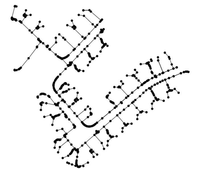
Figure 5: Single-line diagram for the IEEE European low-voltage test feeder
First, a quasi-dynamic simulation was executed in order to evaluate the performance of the algorithms and their precision with respect to the values reported in 31. Fig. 6 shows the active and reactive power at the main substation for the 1.400 scenarios. The four algorithms returned similar results in terms of nodal voltage despite a significant difference in time calculation.
The voltages in each scenario may be initialized at 1 pu or in the voltage of the previous minute. Fig. 7 shows a comparison between the histograms associated with the iterations of these two approaches. As expected, the initialization in the previous scenario reduces the number of iterations since the initial point is close to the final solution. This, however, is not a significant improvement.
Next, each of the power flow algorithms was evaluated for the scenario t= 566min, which corresponds to the maximum load. The convergence plot is depicted in Fig. 8. As expected, the fixed-point method and backward-forward sweep algorithm exhibit exactly the same behavior. The same can be said for Newton’s method in the conventional real and complex domains. There are minor differences in the last iteration, which are related to rounding errors, considering the large set of matrices that require inverse calculation in Newton’s method.
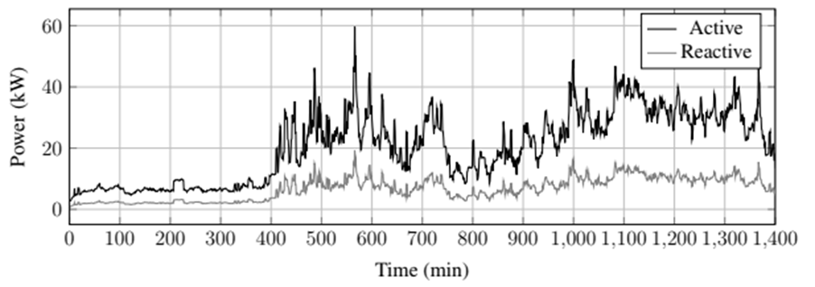
Figure 6: Active and reactive power in the substation for the IEEE 900-node test system using quasi-dynamic simulation

Figure 7: Histogram of the number of iterations with initialization at 1 pu and initialization in the last scenario
While convergence in the fixed-point methods is linear, convergence in Newton’s methods is quadratic. Therefore, Newton’s methods have a faster convergence in terms of iterations. However, the proposed algorithms have very different calculation time. The backward-forward sweep method has the fastest time, followed by its equivalent, the fixed-point method with the Ybus formulation. Newton’s method has the highest time, especially in the complex domain formulation. Table I shows the calculation times for each algorithm. This time was obtained using Matlab’s online application.
Table I: Comparisons between different power flow methods for IEEE European Low-Voltage System
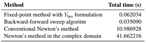
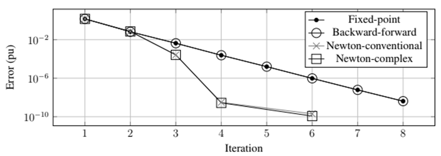
Figure 8: Convergence plot for different power flow algorithms
The fixed-point algorithm with Ybus requires slightly more time. However, it deals directly with meshed grids, and it may be a good option in practice.
Conclusions
This paper revisited the power flow problem in power distribution networks while including theoretical and practical aspects. Four power flow methods for three-phase unbalanced power distribution networks were evaluated, namely the conventional Newton’s method, Newton’s method in the complex domain, the fixed-point method with Ybus representation, and the backward-forward sweep algorithm. It was demonstrated that both Newton’s methods were equivalent. In addition, quadratic convergence and uniqueness of the solution may be ensured by these methods. Likewise, it was demonstrated that the fixed-point method and the backward-forward algorithm are equivalent. Linear convergence of these algorithms was demonstrated both theoretically and numerically.
Newton’s methods require less iterations than the fixed-point methods. However, each iteration in the fixed-point methods is faster. Therefore, fixed-point methods are preferred in practice for power distribution networks.
A Matlab toolbox was also developed. This toolbox may be used for teaching and research. Its functions allow the calculation of three-phase unbalanced power distribution networks with different load profiles. It is easy to modify the functions in order to include renewable power generation, voltage regulators, electric vehicles, and any other new distributed component.
Acknowledgements
Acknowledgment
This work was partially funded by the project project Integra2023, code 111085271060, contract 80740-774-2020, by the Ministry of Science, Technology, and Innovation (Minciencias), and the project ODiN (Optimal Operation of Distribution Networks).
References
Appendix
A. Matlab functions
A toolbox of Matlab functions was created to evaluate the power flow methods. The code of these functions is open-source, so that it may be helpful for future research. The code can be downloaded at (30). It uses only the standard Matlab function as well as the functions xlsread() for reading Excel files and sparse() for creating sparse matrices. This toolbox may also be used to evaluate other three-phase unbalanced systems if the input information is stored correctly. The input file is an Excel workbook with six worksheets. The information required in each worksheet is presented below:
• Worksheet name: general. It contains general information of the test system. At least, the following information is required:
1. Nominal line-to-line voltage in kV
2. Nominal power in MW
• Worksheet name: lines. It contains the connection of the feeder with the following columns:
1. Bus 1
2. Bus 2
3. Length (m)
4. Line code (a number referring to the worksheet line codes)
• Worksheet name: line codes
1. Identification number
2. R1 (Ohm/km)
3. X1(Ohm/km)
4. R0(Ohm/km)
5. X0(Ohm/km)
• Worksheet name: loads.
1. Bus
2. phase (1 for A, 2 for B and 3 for C)
3. power factor
4. Profile (a number referring to the worksheet profiles)
• Worksheet name: profiles. Each column of this worksheet contains a set of active power for the corresponding load.
• Worksheet name: coordinates. It contains the coordinates for piloting the system’s graph. It contains the following information:
1. Bus
2. x coordinate
3. y coordinate
The toolbox contains the following basic functions:
• load feeder.m: It reads the excel file, organizes the information, and calculates per-unit equivalents
Input : a string with the name and address of the workbook
Output : a struct with the following fields:
1. graph: coordinates of the nodes
2. z line 3 × 3 × n tensor with the equivalent impedance of each line in per unit
3. ybus: n × n three-phase nodal admittance matrix
4. yns: sub-matrix YRS
5. ynn: sub-matrix YRR
6. znn: inverse of YRR
7. loads: table of loads
8. profiles: table of profiles
9. xy: node coordinates
10. vs initial: initial voltages for the slack node
11. vn initial: initial voltages for the remaining voltages
12. p base: nominal phase power
13. v base: nominal line-to-neutral voltage
14. n slack: slack nodes for each phase
15. nother: list of remaining nodes
16. num n: number of nodes
17. num l: number of lines
18. num d: number of loads
19. num e: number of profile scenarios
• load flow newton.m: It solves the power flow using conventional Newton’s method
Input : struct generated by load feeder.m and profile scenario
Output : struct with the following information:
1. v node: vector of nodal voltages
2. s node: vector of nodal powers
3. error: error in each iteration
4. iter: total iterations
5. scenario: scenario number
• load flow sweep.m: load flow using the backward-forward sweep method. Same input and output information as load flow newton.m.
• load flow scl.m: load flow using Newton’s method in the complex domain. Same input and output information as load flow newton.m.
• load flow ybus.m: load flow using the fixed-point method with Ybus representation. Same input and output information as load flow newton.m.
• show results.m: it shows a table with nodal voltages and powers, and it plot the feeder’s graph.
License
Copyright (c) 2022 Alejandro Garcés-Ruiz

This work is licensed under a Creative Commons Attribution-NonCommercial-ShareAlike 4.0 International License.
![]()
From the edition of the V23N3 of year 2018 forward, the Creative Commons License "Attribution-Non-Commercial - No Derivative Works " is changed to the following:
Attribution - Non-Commercial - Share the same: this license allows others to distribute, remix, retouch, and create from your work in a non-commercial way, as long as they give you credit and license their new creations under the same conditions.

2.jpg)