DOI:
https://doi.org/10.14483/23448393.18471Published:
2022-01-04Issue:
Vol. 26 No. 3 (2021): September - DecemberSection:
Sección Especial: Mejores artículos extendidos - WEA 2021SSOP Three-Dimensional Reconstruction of Tibia and Fibula for Applications in Biomechanical Fracture Models
SSOP Reconstrucción tridimensional de la tibia y el peroné para su aplicación en modelos biomecánicos de fracturas
Keywords:
biomechanical models, fibula, 3D reconstruction, tibia (en).Keywords:
modelos biomecánicos, peroné, reconstrucción 3D, tibia (es).Downloads
References
OMS, “Accidentes de trânsito,” 2018. https://www.who.int/es/news-room/fact-sheets/detail/road-traffic-injuries (ac-cessed Jul. 13, 2021).
K. Gichuhi, “Injury Pattern Among Non-fatal Road Traffic Crash Victims,” East Afr. Orthop. J., vol. 1, no. 1, pp. 23-25, 2010. https://doi.org/10.4314/eaoj.v1i1.49454 DOI: https://doi.org/10.4314/eaoj.v1i1.49454
R.-H. Pan et al., “Epidemiology of Orthopedic Fractures and Other Injuries among Inpatients Admitted due to Traffic Accidents: A 10-Year Nationwide Survey in Taiwan,” Sci. World J., vol. 2014, ID. 637872, Feb. 2014. https://doi.org/10.1155/2014/637872 DOI: https://doi.org/10.1155/2014/637872
J. D. Heckman and J. Sarasohn-Kahn, “The economics of treating tibia fractures. The cost of delayed unions,” Bull. Hosp. Jt. Dis., vol 56, No 1, pp 63-72, 1997. https://pubmed.ncbi.nlm.nih.gov/9063607/
D. Wennergren, C. Bergdahl, J. Ekelund, H. Juto, M. Sundfeldt, and M. Möller, “Epidemiology and incidence of tibia fractures in the Swedish Fracture Register” Injury, vol. 49, no. 11, pp. 2068-2074, Nov. 2018. https://doi.org/10.1016/j.injury.2018.09.008 DOI: https://doi.org/10.1016/j.injury.2018.09.008
E. Meinberg, J. Agel, C. Roberts, M. D. Karam, and J. F. Kellam, “Fracture and Dislocation Classification Compendium–2018,” J. Orthop. Trauma, vol. 32, no. 1, Jan. 2018. https://doi.org/10.1097/bot.0000000000001063 DOI: https://doi.org/10.1097/BOT.0000000000001063
S. H. Khan, A. J. Ahmad, and M. Umar, “Tibial Plateau Fractures: A New Classification Scheme,” Clin. Orthop. Rel. Res., vol 375, pp. 231-242, Jun. 2000. https://pubmed.ncbi.nlm.nih.gov/10853174/ DOI: https://doi.org/10.1097/00003086-200006000-00028
H. Sun, Q. F. He, B. Bin Zhang, Y. Zhu, W. Zhang, and Y. M. Chai, “¿A biomechanical evaluation of different fixation strategies for posterolateral fragments in tibial plateau fractures and introduction of the ´magic screw`, Knee, vol. 25, no. 3, pp. 417-426, Apr. 2018. https://doi.org/10.1016/j.knee.2018.03.015 DOI: https://doi.org/10.1016/j.knee.2018.03.015
Nelson, V., Deshpande, S., Gray, A. et al. “Comparison of digitally reconstructed radiographs generated from axial and helical CT scanning modes: a phantom study,” Australas. Phys. Eng. Sci. Med., vol. 37, pp, 285-290, Mar. 2014. https://doi.org/10.1007/s13246-014-0257-x DOI: https://doi.org/10.1007/s13246-014-0257-x
A. Tsaturyan et al. “Technical aspects to maximize the hyperaccuracy three-dimensional (HA3D™) computed tomog-raphy reconstruction for kidney stones surgery: a pilot study,” Urolithiasis, vol. 49, pp. 559-566, Apr. 2021. https://doi.org/10.1007/s00240-021-01262-6 DOI: https://doi.org/10.1007/s00240-021-01262-6
J. Huo et al., “Value of 3D preoperative planning for primary total hip arthroplasty based on artificial intelligence tech-nology,” J. Orthop. Surg. Res., vol. 16, art. no. 156, Feb. 2021. https://doi.org/10.1186/s13018-021-02294-9 DOI: https://doi.org/10.1186/s13018-021-02294-9
G. Marongiu, R. Prost, and A. Capone, “Use of 3D modelling and 3D printing for the diagnostic process, decision making and preoperative planning of periprosthetic acetabular”, BMJ Case Rep., 13, no. 1, art no. e233117., Jan. 2020. https://doi.org/10.1136/bcr-2019-233117 DOI: https://doi.org/10.1136/bcr-2019-233117
C. J. Tan, W. C. H. Parr, W. R. Walsh, M. Makara, and K. A. Johnson, “Influence of Scan Resolution, Thresholding, and Reconstruction Algorithm on Computed Tomography-Based Kinematic Measurements”, J. Biomech. Eng., vol. 139, no. 10, art. no. 28787471, Oct. 2017. https://doi.org/10.1115/1.4037558 DOI: https://doi.org/10.1115/1.4037558
J. Aldrich et al., Dose Reduction in CT while Maintaining Diagnostic Confidence: A Feasibility/Demonstration Study, Vienna, Austria: International Atomic Energy Agency, 2009. https://www-pub.iaea.org/MTCD/Publications/PDF/te_1621_web.pdf
D. J. Brenner, “Computed Tomography — An Increasing Source of Radiation Exposure”, N. Eng. J. Med., vol. 357, no. 22, pp. 2277- 2284, Nov. 2007. https://dx.doi.org/10.1056/NEJMra072149 DOI: https://doi.org/10.1056/NEJMra072149
K. Matsiushevich, C. Belvedere, A. Leardini, and S. Durante, “Quantitative comparison of freeware software for bone mesh from DICOM files,” J. Biomech., vol. 84, pp. 247-251, Feb. 2019. https://doi.org/10.1016/j.jbiomech.2018.12.031 DOI: https://doi.org/10.1016/j.jbiomech.2018.12.031
Materialise, “CT scan protocol leg 3 regions”, 2017. https://www.materialise.com/en/resources/all/scan-protocols (ac-cessed Jul. 13, 2021).
Aloopingicon, “Stuff: Measuring the difference between two meshes”, 2010. http://meshlabstuff.blogspot.com/2010/01/measuring-difference-between-two-meshes.html (accessed Jul. 13, 2021).
Mimics, “Mimics Student Edition Course Book”, 2021. https://www.materialise.com/en/medical/mimics-innovation-suite/academic-research-education (accessed Jul. 13, 2021).
3DSlicer, “Documentation/4.10”, 2021. https://www.slicer.org/wiki/Documentation/4.10 (accessed Jul. 13, 2021).
How to Cite
APA
ACM
ACS
ABNT
Chicago
Harvard
IEEE
MLA
Turabian
Vancouver
Download Citation
Recibido: 15 de agosto de 2021; Aceptado: 15 de septiembre de 2021; Recibido: 15 de agosto de 2021; Revisión recibida: 27 de agosto de 2021; Aceptado: 15 de septiembre de 2021
Abstract
Context:
Non-fatal injuries represent a public health issue. Among them, lower limb fractures have a large impact on the costs related to orthopedic treatments. In this work, a three-dimensional reconstruction of the tibia and fibula was performed for biomechanical applications with the purpose of defining the 3D reconstruction parameters that allow reducing patients’ radiation exposure and computational costs.
Method:
For the 3D reconstruction, a computerized tomography taken from a volunteer was used, as well as two software applications specialized in DICOM image reconstruction (Mimics Research and 3DSlicer). The number of images included in the volume was modified, and the results were compared. The quality of the reconstructed volumes was verified by comparing the reference volume reconstructed with the total number of images/slices vs. the modified volumes. The MeshLab software was used for this purpose. The analyzed parameters were the distance differences between the reference and the alternative models, as well as the qualitative curvature analysis.
Results:
The ANOVA results for the Max (maximum distance between meshes) response shows that software and slices are significant factors. However, the software-slices interaction did not have a significant influence. As for the RMS (root mean square) distance response, software, slices, and the softwareslices interaction are not significant. For the Mean distance response, slices and the software-slices interaction are not significant. Nevertheless, software significantly influences the response. These result suggest a potential way to reduce the computational cost and the patient’s radiation exposure in future biomechanical and preoperatory analyses, since the same quality can be obtained by including fewer 2D
images in the reconstruction.
Conclusions:
The reconstructed surfaces are smoother when Mimics is used, even though the same smoothness factor was employed in both software applications during the reconstruction. When 16 slices are used (retained every 16 images from the complete original model), the distance differences increased for both bones (tibia and fibula). For the RMS, reducing the number of slices and using either one of the two applications analyzed would not show any significant differences in the reconstruction, thus allowing the potential reduction of radiation exposure of the patient.
Keywords:
biomechanical models, fibula, 3D reconstruction, tibia.Resumen
Contexto:
Las lesiones no fatales representan un problema de salud pública. Entre ellas, las fracturas de las extremidades inferiores tienen un gran impacto en los costos relacionados con los tratamientos ortopédicos. En este trabajo se realizó una reconstrucción tridimensional de la tibia y el peroné para aplicaciones biomecánicas con el fin de definir los parámetros de reconstrucción 3D que permitan reducir la exposición a la radiación de los pacientes y el costo computacional.
Método:
Para la reconstrucción 3D se empleó una tomografía computarizada tomada a un voluntario. Se utilizaron dos programas de software especializados en la reconstrucción de imágenes DICOM (Mimics Research y 3DSlicer). Se modificó el número de imágenes 2D incluidas en el volumen y se compararon los resultados. La calidad de los volúmenes reconstruidos se verificó comparando el volumen de referencia reconstruido con el número total de imágenes/cortes frente a los volúmenes modificados. Para ello se utilizó el software MeshLab. Los parámetros analizados fueron las diferencias de distancia entre el modelo de referencia y el alternativo, y el análisis cualitativo de la curvatura.
Resultados:
Los resultados del ANOVA para la respuesta Max (distancia máxima entre mallas) muestran que el software y los cortes son factores significativos. Sin embargo, la interacción software-cortes no tuvo una influencia significativa. Para la respuesta RMS (Root Mean Square) el software, los cortes y la interacción software*cortes no son significativos. Para la respuesta media, los cortes y la interacción software-cortes no son significativos. Sin embargo, el software influye significativamente en los resultados Estos resultados suponen una reducción del coste computacional y de la exposición de los pacientes a radiación en futuros análisis biomecánicos y preoperatorios, ya que se puede obtener la misma calidad incluyendo menos imágenes 2D en la reconstrucción.
Conclusiones:
Las superficies reconstruidas son más suaves cuando se utiliza Mimics a pesar de que se utilizó el mismo factor de suavidad en ambos programas durante la reconstrucción. Cuando se utilizan 16 cortes (retenidas cada 16 imágenes del modelo original completo), las diferencias de distancia aumentan para ambos huesos (tibia y peroné). Para el RMS, reducir el número de cortes y utilizar cualquiera de los dos programas analizados no presentaría diferencias significativas en la reconstrucción planteándose como una forma potencial para la reducción de la exposición a la radiación del paciente.
Palabras clave:
modelos biomecánicos, peroné, reconstrucción 3D, tibia..Introduction
The World Health Organization (WHO) defines non-fatal injuries as a public health problem [1].Within these traumas, tibia injuries have been demonstrated to be one of the most common. Epidemiological studies worldwide report that this type of injury represents the largest number of fractures, which can be attributed to traffic accidents affecting the lower limbs [2], [3]. Moreover,the National Institute of Forensic Medicine reported tibia fractures as the third most prevalent pediatric injury. According to the data reported by the WHO, on an annual basis, between 20 and 50 million people in the world suffer non-fatal injuries due to traffic accidents, highlighting lower limb fractures as a public health problem. Hence, repairing lower limb fractures greatly impacts the costs related to orthopedic treatments around the world. [4], [5] indicate that the leading causes of tibial fractures in developed countries like Sweden between 2011 and 2015 were simple falls (44 %) and traffic accidents (22 %). Tibial fractures can be classified according to their location and type of injury. The Orthopedic Trauma Association and the AO Foundation classified these fractures by location and morphology, and they provided additional classifications related to open, pediatric, and eriprosthetic fractures [6]. Tibial plateau fractures are prevalent, and they have been divided into several groups: lateral and medial tibial plateau fractures, posterior tibial plateau fractures, coronal splits, bicondylar fractures, and under subcondylar fractures [7]. The type of treatment is selected based on the surgeon’s experience, and, in some cases, the result can be subjective. Another option to select and evaluate the fixation geometry is the use biomechanical models, which are developed based on a 3D reconstruction of fractured bones.
Biomechanical models allow evaluating and predicting the behavior of potential fixation configurations in different types of fractures using computer simulation and laboratory tests [8]. Computational models also aid in making several therapeutic decisions, such as patient positioning for radiotherapy treatments [9], kidney stones surgery [10], and preoperative orthopedic planning processes [11], [12]. The construction of biomechanical models starts with the acquisition of a stack of 2D cross-sectional medical images (i.e., computerized tomography, CT), which are then volumetrically represented and used in numerical computational analyses. Therefore, improving the image acquisition protocols would provide safer and more cost-effective processes. Experimental analysis of the influence of scan resolution, thresholding, and reconstruction algorithm on CT-based kinematic measurements [13] showed no significant influence on the accuracy of the calculated bone kinematics. Therefore, a lower resolution scan was recommended, which is one of the physical parameters to optimize the quality of the image for it to be good enough to perform a clinical diagnostic or a 3D reconstruction while keeping the patient’s radiation exposure as low as possible [14].This is especially important since low-dose radiation exposure due to the increasingly common use of CT has been associated with a potential increased risk of cancer in patients, especially in children [15].
As mentioned above, the first step to developing a biomechanical model is reconstruction using a 2D stack of tomographic images in a medical image analysis software (such as Mimics or 3DSlicer). Previous reports [16] have found minimum differences when the reconstruction is carried out using different free software applications, which obtained bone models of good quality. The authors postulated that freeware is suitable for 3D bone model reconstruction. In this work, a commercial (Mimics Research 19.0, research license) and free software (Slicer, version 4.11) were included in the analysis to study the offer of computational tools and their compliance with quality standards This paper aims to evaluate the configurations used for 3D reconstructions in the tibia and fibula for applications in biomechanical fracture models. This evaluation includes the advantages and disadvantages of two software applications, as well as the number of slices required for quality reconstruction, aiming to reduce the potential exposure dose to radiation.
Experimentation
Acquisition of 2D cross-sectional medical images for 3D reconstruction
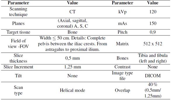
Tomography images were taken from an individual male, who was 25 years old and 1,82 m tall, with a weight of 80 kg and no reported pathologies. Before the image acquisition, the volunteer filled out an informed consent. He was chosen to be used in future studies since his results could be compared to previously collected data available in Opensim databases. The tomographic images were taken using the parameters shown in Table I, based on the CT scan protocol provided by Materialise [17].
Table I: Parameters obtained for the CT scan
Selection of reconstruction software
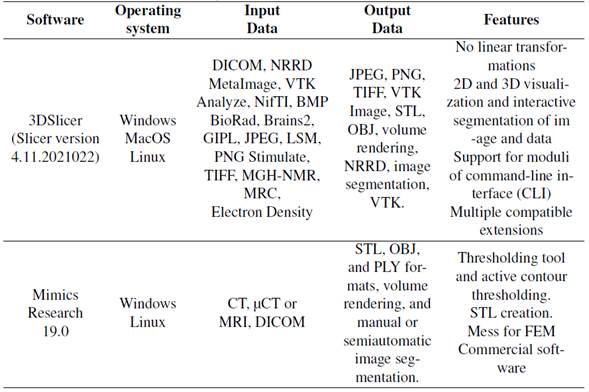
Two software applications with similar capabilities were selected because they were readily available for the study. The selected software was Mimics Research 19.0 (research license) and 3DSlicer (Slicer version 4.11.20210226, open source). The capabilities of the both applications are shown in Table II.
Table II: Capabilities of two software used in this study
Modeling the tibia
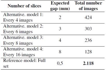
The total number of 2D cross-sectional images (slices) acquired during the CT scan was 2.118.After obtaining the data, the reference model was reconstructed. Alternative models were also reconstructed, creating gaps between the 2D slice files. Table III shows the different number of slices (retained slices from the reference model) used to reconstruct the alternative models. The model’s total number of images/slices considered the helicoidal scanning mode, and the same number was used for both software applications.
Table III: Parameters using different software
The general operation principle was similar in both applications, including importing the DICOM files. The threshold values with a minimum of 124 HU and a maximum of 3.071 HU were used.Image segmentation was performed using various tools that met the same objectives in both Mimics and 3D Slicer. A smooth factor of 0,4 was performed in two iterations, as well as minimal intervention of manual segmentation of the mask. A schematic representation of the steps used to obtain the model is shown in Fig. 1.

Figure 1: Schematic representations of the steps used to obtain the volumetric model
Analysis of reconstructed tibias and fibulas
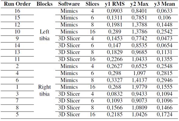
factorial design was used to analyze the effect of two factors: software and the number of slices in the RMS (root mean square), Max (maximum distance between meshes), and Mean distance responses. The responses were obtained via the Euclidean distance of the model with a reduced number of slices vs. the control (the model with the complete number of slices). The MeshLab software was used to calculate the Hausdorff distance, which refers to the maximum distance between two subsets of points, where one belongs to an x-mesh, and the other belongs to a y-mesh.MeshLab samples each point belonging to the x-mesh and takes the closest point of the y-mesh. Therefore, it is very important to perform a previous alignment process between the meshes as accurately as possible. It is also essential to take as many points as possible when applying the filter, which can be ensured by sampling the vertices, edges, and faces [18]. The software factor had two levels: Mimics and 3D Slicer. The number of slices factor had four levels: 4, 6, 8, and 16. The alternative reconstructed models were compared with the reference model, and the right tibia and left tibia were considered as replications. The experimental setup is shown in Table IV. Residual plots were used to test the normality, independence, and constant variance assumptions (data not shown). Outliers identified via scatter plots were extracted from the analysis. The incidence of the effects and two-level interactions was evaluated via ANOVA (p <0,05).
Table IV: Experimental setup for the factorials design
Results and discussion
From the p-values, software (p = 0,02) and slices (p = 0,007) are significant for the response. The software affects the Max of the calculated distances because the line is not horizontal. Moreover,the Mimics software has a higher Max value than 3D Slicer. The number of slices also affects the Max, and, as observed in Figs. 2c and 2d, the highest number was obtained when extracting 16 slices. The overall mean is marked in the dotted reference line. As seen in Fig. 2d, 3DSlicer reports lower Max values in most cases related to slices. However, the p-value (0,060) reveals that this interaction is not significant. The ANOVA results for Max RMS and Mean can be seen in appendix Tables SI, SII, and SIII, respectively.
Figs. 2a and 2b show the Mean effects and interaction plots, respectively. As observed, 3DSlicer has lower RMS values than Mimics, and the higher RMS was noticed with the 16 slices. However,from the p-values, software (p = 0,07), slices (p = 0,24), and the interaction between software and slices (p = 0,97) are not significant for the RMS response. On the other hand, the highest mean value was observed for the model with 8 slices (Figs. 2e and 2f). However, slices (p = 0,56) and the software-slices interaction (p = 0,95) are not significant for the response. Nevertheless, software (p= 0,046) significantly influences the response, and 3DSlicer had a lower Mean value than Mimics.
Visible differences are spotted in the 3D images when using both reconstruction software applications.Fig. 3 shows the reference model for Mimics and its corresponding 3DSlicer reconstructions.The first interesting change is related to the visual smoothness of the surface. Generally speaking,the surfaces are smoother when using Mimics, even though the same smooth factor was used in 3DSlicer. There are indeed differences in the smoothing algorithms. The wrapping tool in Mimics deletes rough areas and gaps in the model, which is especially useful in numerical analyses [19].Since the 2D cross-sectional images were acquired using the helical mode, the removal of images considered potential helicoidal artifacts. On the other hand, the smoothing process in 3DSlicer consists of the remotion of small extrusions and the filling of small gaps without changing the smooth contours [20]. Additionally, Boolean operations were used in 3DSlicer to simulate the wrapping tool in Mimics.
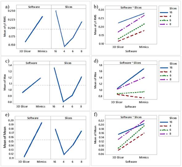
Figure 2: Main effects and interaction plots for RMS, Max, and Mean
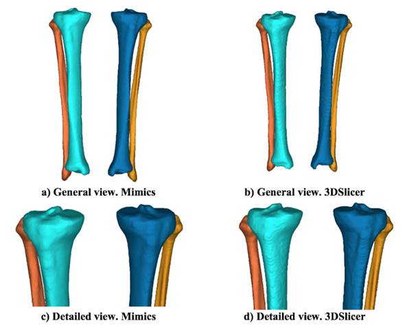
Figure 3: Reference model after reconstructions: a) and c) Mimics; b) and d) 3DSlicer
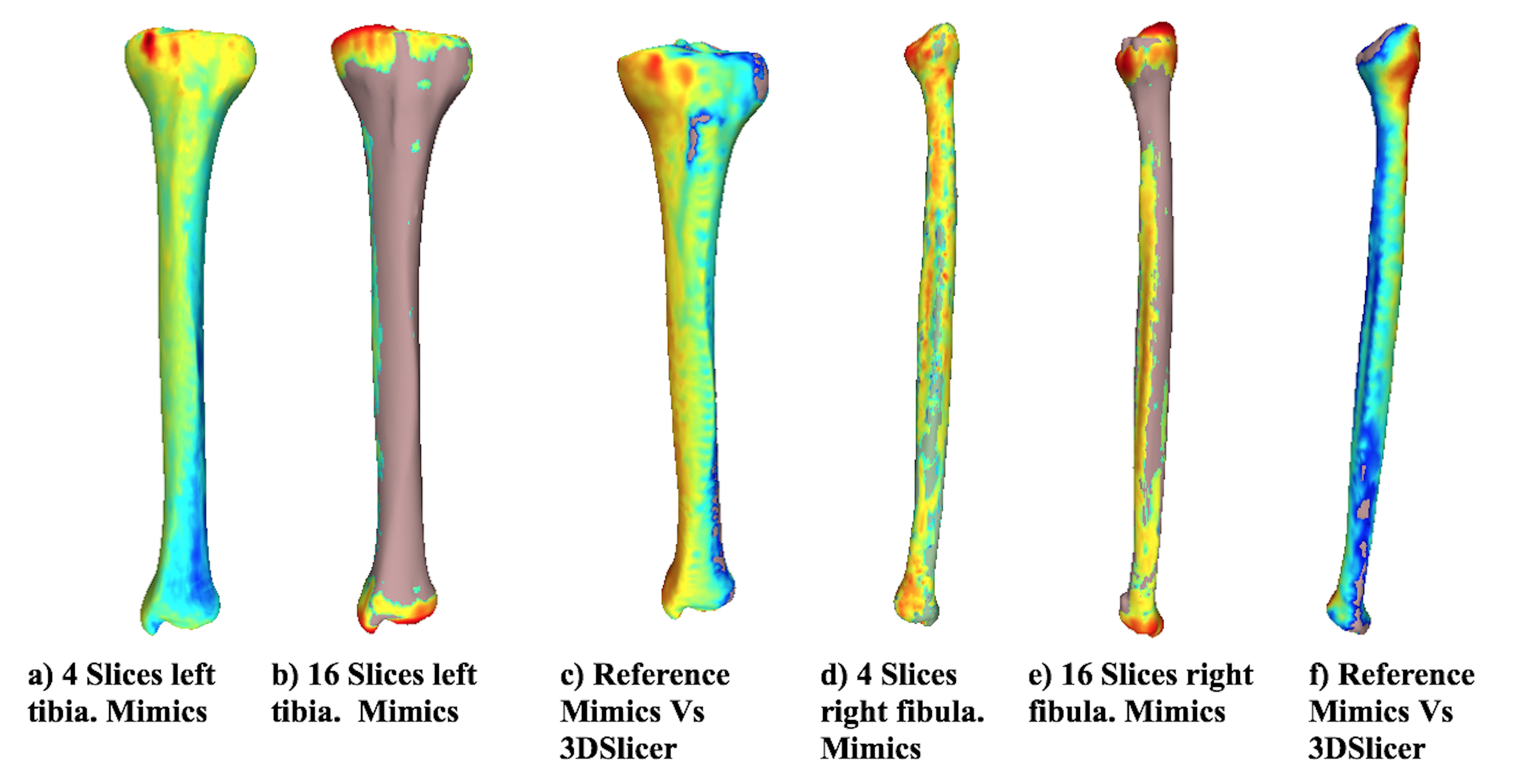
Fig. 4 shows the distance differences from the reference model for both bones using Mimics for the most representative alternative models. In addition, the distance difference between the reference models and the alternative models obtained using each software is shown. When the distance between the two models is larger, the color tends towards red, and when the vertex is close, the color tends to be blue. The chromatic scale defines the intermediate values. The results suggest that the distances between the reference model and the alternative model are neglectable when using 4 slices in the reconstruction. However, with 16 slices, the differences increased, as shown in the changes in the color scale (from blue to red) around the tibia and fibula. The greatest differences (red) in all cases are located at the proximal tibia, given that the complexity of the geometry increases in that area (the tibial plateau). When the two applications are compared, the visual differences are concentrated at the image’s top-left area (proximal zone) for the tibia and at the top-right for the fibula. However, along the length of the bone, the model turns blue, meaning that the reconstruction of each software is very similar. Moreover, the reference model has been colored for comparison purposes. The zones at the Figure that do not have a chromatic scale indicate that, locally, the reconstructed model is larger than the reference model.
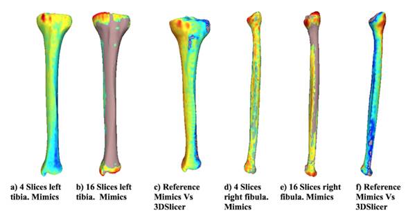
Figure 4: Distance from the reference model
Figure 5 shows the curvature analysis for the left tibia and right fibula alternative models, as well as the reference models using both Mimics and 3DSlicer. The greatest curvature value displayed is 1, and the smallest one is 0,0010. As the radius of curvature decreases, color changes from black (0,0010) to blue, green, and red (1,0000). As the radius of curvature increases, the curvature value decreases. A planar surface has a curvature value of zero because the radii of flat faces are infinite.The results showed that there are no noticeable differences between the reference model and the model reconstructed using 4 slices (not shown). However, when 16 slices are used to reconstruct the alternative model, the curvature (and the continuity) of the surfaces is affected.
Another important difference between the reference and alternative models (16 slices) are compared is the mesh size (element size) in the STL file. When 16 slices are used, the software (Mimics) cannot provide continuity for the surfaces, and some empty elements can be identified (see the empty element in black in Fig 5b at the top-right). When the number of slices is 16, the wrapping tool should be modified as slices are removed. However, in this work, the same wrapping tool was used for comparison purposes. The same behavior was identified for the tibia and fibula, where several empty elements can be observed in Fig. 5d.

Figure 5: Curvature analysis for different numbers of slices (tibia and fibula)
The alternative model (16 slices) for the fibula shows that the mesh size is extremely large, and it does not properly describe the curvature in the proximal zone of the fibula. On the contrary, the curvature along the shaft of the fibula is very similar since the geometry is less complex than the fibular head. Figs. 5e and 5f show the reference model reconstructed using 3DSlicer. The first interesting result is related to the size of the elements. The mesh created using the same procedure in Mimics provides a reference model with more details in the proximal zone of both bones. The curvature is similar for the model reconstructed using Mimics for the proximal zone. However, the surfaces are smoother when reconstructed using Mimics.
To summarize, in this work, the differences between the two software applications were investigated to create STL bone models. The manual intervention by the operator was limited as much as possible by using the same processing parameters, even though the segmentation algorithms of this software are not known. Another important detail related to the processing performed in order to obtain an STL file is that, when the model is exported using the ASCII file, the imported model is less prone to show errors in MeshLab. The same behavior has been reported by other authors [16] In this work, the mesh parameters, such as the number and density of the triangles in the mesh,were only qualitatively specified. Future work could focus on quantifying the parameters of the mesh after the final file is generated. This result suggests that the individual physical size of the triangles depends on the analyzed bone (tibia or fibula).
Conclusions
This work revealed that the software-slices interaction did not significantly influence any of the analyses. The main effects and interaction plot showed that the highest differences were observed in the 16-slice model for the tibia with the RMS and Max analysis. Furthermore, the reconstructed surfaces were smoother when Mimics was used, even though the same smooth factor was used in both software applications during the reconstruction. Nevertheless, Mimics reported continuity issues, and it had the highest RMS and Max.
As for the RMS distance, reducing the number of slices and using either of the applications analyzed, without nature of proof, would not present a significant difference in the reconstruction allowing for the reduction in radiation exposure and computational cost. However, for the Max distance, the reduced mesh would present a significant difference compared with the original reconstruction.For the Mean distance, the mesh would only be affected by the software used and not by the reduced number of slices.
Acknowledgements
Acknowledgments: The authors are grateful to Universidad Nacional de Colombia for funding the project Estado de esfuerzos en un elemento de osteosíntesis en la consolidación de una fractura de miembro inferior (Stress state in an osteosynthesis element in the consolidation of a lower limb fracture, code H:50195).
References
License
Copyright (c) 2022 Valentina Mejía Gallón, María Camila Naranjo-Cardona, Juan Ramírez, Juan Atehortua Carmona, Juan Felipe Santa-Marin, Samuel Vallejo Pareja, Viviana M. Posada

This work is licensed under a Creative Commons Attribution-NonCommercial-ShareAlike 4.0 International License.
![]()
From the edition of the V23N3 of year 2018 forward, the Creative Commons License "Attribution-Non-Commercial - No Derivative Works " is changed to the following:
Attribution - Non-Commercial - Share the same: this license allows others to distribute, remix, retouch, and create from your work in a non-commercial way, as long as they give you credit and license their new creations under the same conditions.

2.jpg)